3DCNN and Its Combinations: Innovations and MATLAB Code

Introduction

This issue introduces a method for bearing fault diagnosis based on multi-resolution mel analysis using 3DCNN.

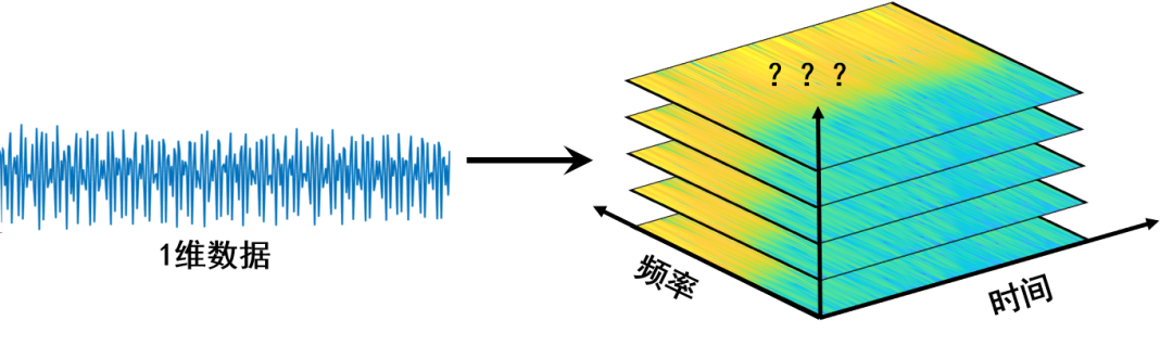
The general idea is to use Mel frequency spectrum analysis to convert one-dimensional fault data into three-dimensional data (as for how to achieve this, it is not convenient to disclose here!) and then input it into the 3DCNN model for training and testing. This experiment was validated on bearing data from Case Western Reserve University and gearbox data from Southeast University, achieving an accuracy of 100%.

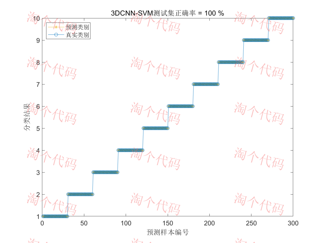
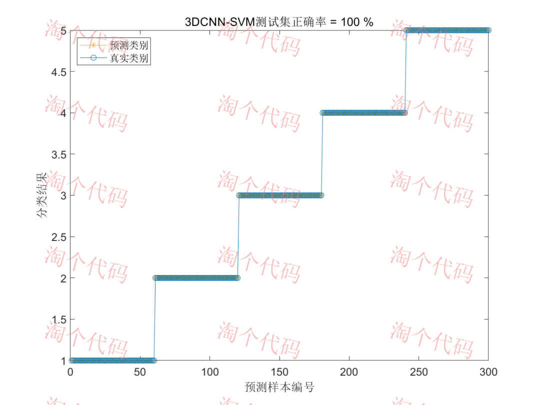
To make the article more substantial, we also integrated the classic 3DCNN-SVM network, which you can choose to use or not.

This method is original to the WeChat public account “Tao Ge Code”; don’t ask, the answer is definitely that no one has used it before!

For those still pondering over innovative points, come and take a look quickly!

The functionality of this code implementation includes:

① Processing of data from Case Western Reserve University and Southeast University gearboxes

② Converting the processed one-dimensional data into three-dimensional data using Mel frequency spectrum analysis (the code also includes a STFT one-dimensional to three-dimensional method for comparison, which can be used or not)

③ Training with 3DCNN

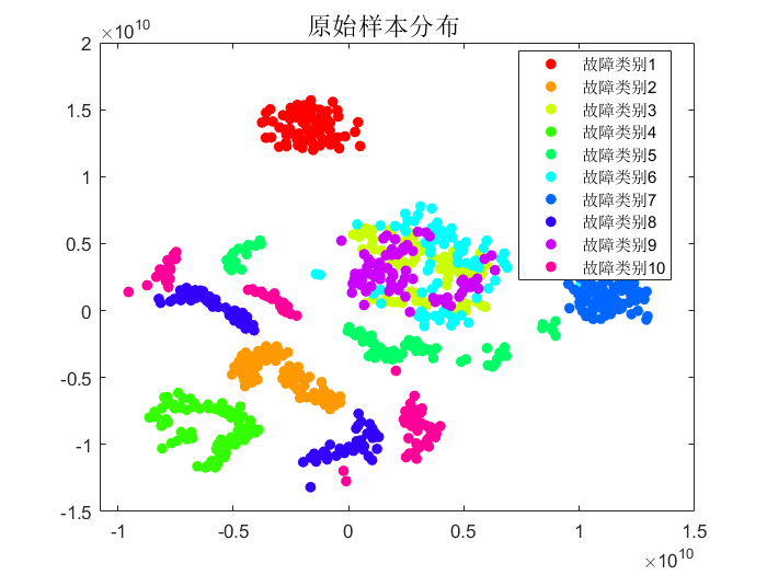
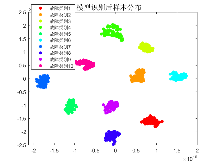
④ Dimensionality reduction analysis using TSEN, with results visualized

⑤ Training and prediction using 3D CNN-SVM (the key here is to learn how to input 3DCNN features into SVM; as long as you know how to input into SVM, you can input into other machine learning classifiers, and combined with some optimization algorithms, a new method is born!)

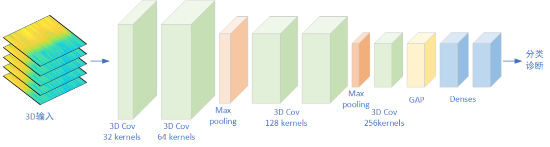
The model structure diagram is as follows (Visio format):

Content Details

1. Data Processing

① Processing the data downloaded from the official website of Case Western Reserve University, the steps are as follows:

1. Load a total of 10 types of data, then take the DE_time of each data (%DE is the drive end data, FE is the fan end data, BA is the acceleration data; just choose one)

2. Set the sliding window w, the number of fault sample points s for each data, and the sample size m for each fault type

3. After sliding all the data, combine them into a single data variable

4. There have been previous articles discussing the processing of Case Western Reserve University data; you can refer to this article: Processing of Case Western Reserve University Bearing Diagnosis Data, Free MATLAB Code Available

   The final data is a 1000*2048 matrix, where 1000 is the sample size and 2048 is the features. 1000 equals 100*10, where 10 refers to 10 fault states, and 100 refers to 100 samples for each state. In the code, it is data_total_1797.mat

② Processing the data downloaded from the official website of Southeast University, the steps are as follows:

1. Load a total of 5 types of gearbox data, selecting the one with a speed of 20Hz (or 1200rpm) – load 0V(0Nm) under 5 types of fault data:

   Chipped tooth (gear with cracks)

   Normal operation (Health working state)

   Missing tooth

   Root fault (crack at the root of the gear)

   Surface fault (wear on the tooth surface)

2. Set the sliding window w, the number of fault sample points s for each data, and the sample size m for each fault type

3. After sliding all the data, combine them into a single data variable

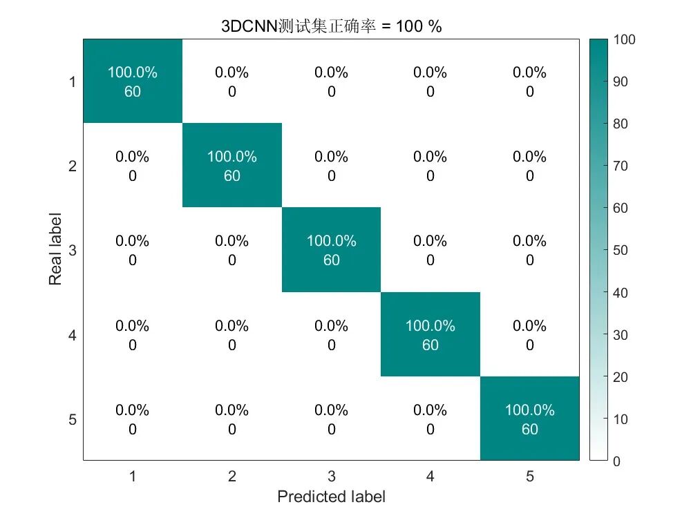
4. The final data is a 1000*2048 matrix, where 1000 is the sample size, with 200 samples taken for each fault, and 2048 is the features. 1000 equals 200*5, where 5 refers to 5 fault states, and 200 refers to 200 samples for each state. In the code, it is data_total.mat

2. Performing Mel Frequency Spectrum Transformation on the Data

The transformed data consists of a series of 3D data, with the first row being the data itself and the second row being the label column.

3. Results Presentation

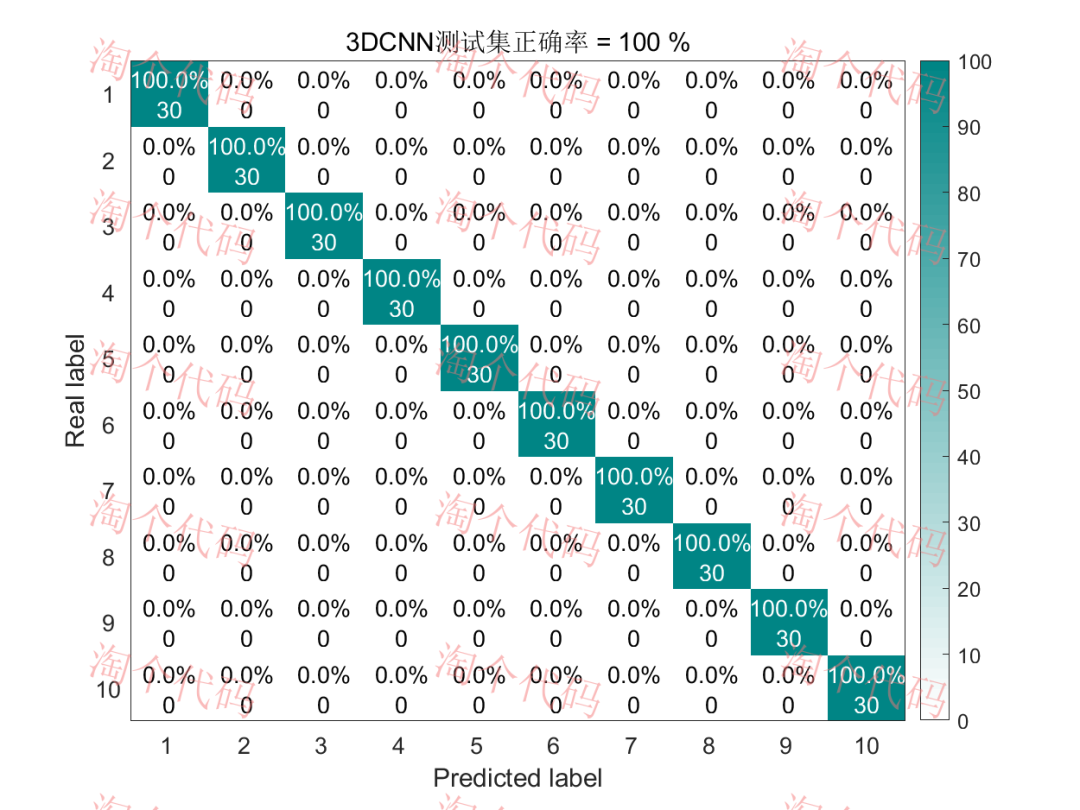
Diagnosis results for Case Western Reserve University bearing data (the first 70 samples of each group are used for training, and the last 30 for testing):

Diagnosis results for Southeast University gearbox data (the first 140 samples of each group are used for training, and the last 60 for testing):

The network structure of 3DCNN is as follows: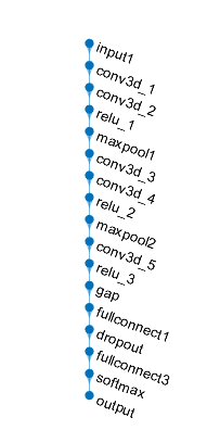

Each folder of this program code contains a description.txt; please read it carefully before running, as it will help you better understand the program. Steps can be executed one by one.

I hereby promise that the above experiments are all real and valid!

Code Directory

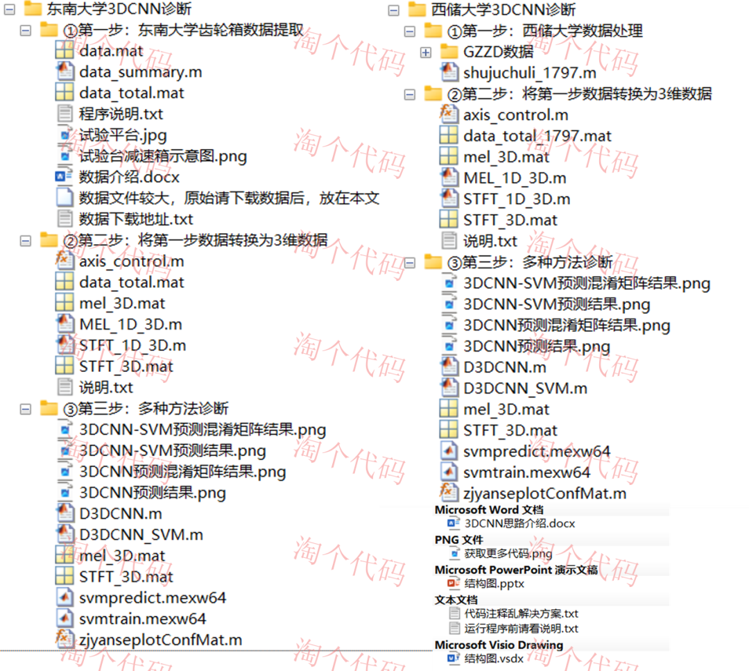Accompanying document description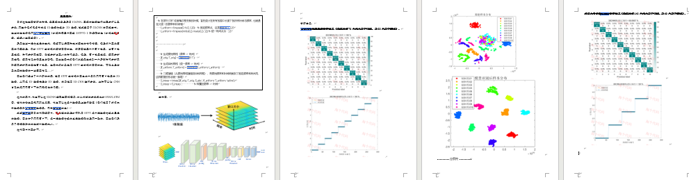

Code Acquisition

Link:https://mbd.pub/o/bread/aJWXmZtr