
Jishi Guide
Big questions about the popular LoRA in the model training community! Dive deep into understanding LoRA with source code analysis.>> Join the Jishi CV Technology Group to stay at the forefront of computer vision.
Introduction
Since ChatGPT sparked the trend of large language models (LLMs), a wave of LLMs (GPT-4, LLaMa, BLOOM, Alpaca, Vicuna, MPT, etc.) has emerged. They can handle knowledge Q&A, article writing, code writing and debugging, report planning, etc. They can also play word games interactively with you. Some talented friends have even connected LLMs as interactive interfaces to various other modalities (e.g., visual & speech) to create explosive multimodal effects. Amazing!
Such excitement inevitably makes everyone want to create their own dedicated LLM (doesn’t it feel like going back to childhood pet training games?). However, most “civilian” players like CW do not have the resources to play with LLMs (mainly GPUs). Let alone models with hundreds of billions of parameters, even those with tens of billions of parameters are not affordable for many.
For most people, the closest they get to LLMs is running an open-source demo to see the inference process and getting a result that is “expected”. Then, they ironically self-congratulate: WOW~ So impressive! We are one step closer to AGI! As for training one? They would say: Ha ha.. Don’t think too much, go to bed!
A technology usually does not become widely used at the moment of its birth; like humans, it also needs opportunities. The current background has intensified the contradiction of most civilians in the era of large models. Thus, the protagonist of this article, LoRA (Low-Rank Adaptation of Large Language Models), which was born in 2021, has become the popular choice in model training, successfully gaining attention.
This article will first introduce the concept and advantages of LoRA, discuss its motivation and the problems with previous methods, and then explore LoRA from seven aspects in a question-and-answer format (combined with source code analysis). Afterward, we will delve deeper into some aspects of LoRA, and finally provide an example of applying LoRA for fine-tuning. Those who already have a basic understanding of LoRA can jump directly to the sections “Seven Questions about LoRA” and “The Advancing LoRA”.
Tell Me What LoRA Is
In today’s fast-paced world, people tend to be impatient. You’ve heard me ramble on without explaining what LoRA actually is, and you must be eager to know. Oh? You say you don’t know? That’s great, CW gives you a thumbs up! But I won’t dilly-dally, let’s get to the point.
LoRA stands for “Low-Rank Adaptation”. Seeing “low-rank”, those familiar with linear algebra should reflexively think of low-rank matrices. Bingo! That’s exactly what it means. You ask me what LoRA is called in Chinese? Em.. Let’s call it “低秩(自)适应”, although the English version doesn’t have “self”, it conveys the idea of adaptation based on LoRA’s principles and practices.
In summary, LoRA is a technology primarily used for fine-tuning LLMs. It introduces additional trainable low-rank decomposition matrices while fixing the pre-trained weights. The key point of this approach is that: the pre-trained weights do not need training, thus no gradients are computed, and only the parameters of the low-rank matrices are trained.
One thing CW must tell you: the number of parameters introduced by the low-rank matrices is much less than that of the pre-trained weights! This means that compared to full fine-tuning, the number of trainable parameters is significantly reduced, so less GPU memory is required. This is simply wonderful for us civilians!
With LoRA, we can enjoy many benefits, such as:
-
When facing different downstream tasks, only a small number of parameters in the low-rank matrices need to be trained, while the pre-trained weights can be shared across these tasks; -
It eliminates the gradients of the pre-trained weights and related optimizer states, greatly increasing training efficiency and reducing hardware requirements; -
The trained low-rank matrices can be merged into the pre-trained weights, transforming multi-branch structures into single-branch, achieving no inference delay; -
It does not interfere with previous parameter-efficient fine-tuning methods (like Adapter, Prefix-Tuning, etc.), and they can be combined.
Note: Parameter-efficient fine-tuning methods (PEFT) only require tuning a small number of parameters (which can be newly introduced) without fine-tuning all parameters of the pre-trained model, thus reducing computational and storage resources.
Source of Inspiration
For any technology, CW is often curious about the ideas behind its invention. Specifically, where did the inventors get their inspiration? Unfortunately, I can’t interview the authors in person, or I would definitely let them “talk at length”! But I can only find answers through the paper.
CW found that the authors mentioned in the paper: previous works indicate that models are often “over-parameterized”, and during optimization, the parameters that are updated usually “reside” in a low-dimensional subspace. Based on this, the authors naturally hypothesized that the parameter updates of pre-trained models during fine-tuning for downstream tasks also follow this pattern.
Moreover, previous PEFT methods had a series of issues, such as increasing inference delay, increasing model depth, limiting input sentence length, etc. More importantly, most of them performed worse than full fine-tuning, meaning that the final trained model’s performance was not as good as full fine-tuning.
Combining their hypothesis with the current era’s background, the authors created LoRA. The models trained using this approach can ultimately rival the performance of full fine-tuning and even outperform it on some tasks.
Where Previous PEFT Methods Fell Short
In the previous chapter, CW briefly mentioned some issues with previous PEFT methods, and now I will elaborate a bit more.
Before LoRA, the more representative PEFT methods mainly included introducing adapter layers for downstream tasks and optimizing activations close to the model input layer. For the latter, a notable example is prefix tuning. To be fair, these methods are somewhat effective, but they are just not good enough.
For methods that introduce adapter layers, their shortcomings are:
-
The new adapter layers must be processed sequentially, thereby increasing inference delay; -
More GPU synchronization operations are needed during distributed training (like All-Reduce & Broadcast).
As for the other type of methods, using prefix tuning as an example, they fall short in:
-
The method itself is difficult to optimize; -
This method requires reserving a portion of the input sequence as a tunable prompt, thereby limiting the original input text’s sentence length.
Seven Questions about LoRA
The first four sections focus on theoretical analysis, incorporating formulas and experimental results from the paper. The last three sections will include source code analysis for deeper insights.
Why Introduce Low-Rank Matrices?
The authors mentioned that they previously saw a paper: Intrinsic Dimensionality Explains the Effectiveness of Language Model Fine-Tuning. This paper concluded that the weight matrices of pre-trained language models have very low intrinsic rank after fine-tuning on downstream tasks.
【Understanding intrinsic rank】“Intrinsic” directly translates to “inherent” or “intrinsic”, so I saw someone directly call intrinsic rank as “内在秩”. (⊙o⊙)… I find this term a bit awkward and unclear.CW thinks that here, “intrinsic” should be understood as “essential” or “most representative”. Therefore, “intrinsic rank” should be understood as the number of dimensions (features) that best represent the essence of the data, which we can elegantly call “本征秩”. In signal processing, there is also a corresponding concept—intrinsic dimension, which represents the minimum number of features that can represent a signal, corresponding to the features that best reflect the essence of the signal.
In other words, after adapting to downstream tasks, the intrinsic rank of the weight matrix becomes very low, which signifies that such high dimensionality is not necessary for representation, and there is redundancy in the high-dimensional weight matrix.
Based on this, the authors confidently believe that the part of the weights that are updated during fine-tuning must also be low-rank.
Inspired by this, we hypothesize the updates to the weights also have a low “intrinsic rank” during adaptation.
You ask: “What does the part of the weights that are updated refer to?”
CW answers: The changes in weights during the fine-tuning process can be represented as . Here is the weight before updating (initially the pre-trained weight), and is the updated part, which is the amount to be updated calculated after obtaining the gradient through backpropagation.
What Does LoRA Change?
Assume , since gradients and weight parameters are one-to-one, thus . Now, since we believe that the intrinsic rank of is very low, let’s perform a low-rank decomposition:
, where , and .
This is what is called low rank, as it is far smaller than and .
As a result, after low-rank decomposition, the number of parameters in this part is much smaller than that of the pre-trained weights.
Logically, appears in the backpropagation phase, but we can “bring it out early”: let it participate in the forward process together with . In this way, during backpropagation, the gradients will only propagate to this part, as is initially the pre-trained weight, which is fixed and does not require gradients.
After LoRA’s “baptism”, if you feed the model an input , the forward process can be expressed as:
Additionally, two points need to be mentioned:
-
Initialization of low-rank matrices B, AB, A.
After the low-rank decomposition, to maintain the model’s output as that of the original pre-trained model (i.e., without ), we initialize as all zeros, while is randomly initialized with a Gaussian distribution.
-
Scaling the output of the low-rank part .
The authors also mentioned in the paper that for this part, a scale factor will be multiplied. This scale factor maintains a constant relationship with . The authors believe adjusting this is roughly equivalent to adjusting the learning rate, so they simply fix it as a constant (this way, they can be a bit lazy).
Which Part’s Memory Demand Is Reduced?
Since the number of parameters of is much smaller than , LoRA reduces the memory demand for optimizer states compared to full fine-tuning.
This is because the optimizer saves a copy of the model parameters that need to be updated. In the full fine-tuning approach, to update all parameters, the optimizer saves a copy of all parameters; while our lovely LoRA only needs to update this part, so the optimizer saves a copy of parameters only, where is much smaller than .
Additionally, we might easily assume that LoRA’s memory demand for the gradient part is also much less than full fine-tuning. But is this really the case? Let’s analyze how the gradient is computed.
Assuming the model has obtained an output after the forward process as shown in the formula, and we further compute the loss, now we are here to find the gradient of . According to the chain rule, we easily get:
Note that this part is the same as when performing full fine-tuning; the shape of this gradient is consistent with the shape of the weight matrix, both being .
OMG! This means that in the process of computing the gradient of , the memory required is not less than that of full fine-tuning, as it is necessary to compute the gradient matrix with shape . Even more awkwardly, due to the presence of , the memory and computation required during gradient computation may even be greater than full fine-tuning. Fortunately, after the computation is complete, this intermediate state will be released, and we only need to store the gradient matrix with shape .
Thus, for the gradient part, in a strict sense, LoRA cannot reduce its memory demand, and it may even require more computational resources than full fine-tuning, but it reduces the demand for final storage.
Which Parts of the Model Are Decomposed into Low-Rank?
However, in today’s 202x era, models typically have N weight matrices, so which ones should undergo low-rank decomposition? Should we just go all out?
For this question, the authors chose to be lazy and only applied LoRA to the projection matrices in the self-attention layers (e.g.,), while the MLP modules and structures outside the self-attention layers were left “unattended”.
In the Transformer architecture, there are four weight matrices in the self-attention module (Wq, Wk, Wv, Wo) and two in the MLP module.We limit our study to only adapting the attention weights for downstream tasks and freeze the MLP modules.We leave the empirical investigation of adapting the MLP layers, LayerNorm layers, and biases to a future work.
The authors might have guessed that you would ask: Which projection matrices in the self-attention layers should LoRA be applied to? For this question, they did put in some effort to conduct experiments.
In the experiments, the authors used the 175B GPT-3 as the research object and set a budget of 18M for the number of parameters that can be fine-tuned. In this setup, when applying LoRA to only one of the projection matrices in each layer, the rank equals 8; if LoRA is applied to two of the projection matrices in each layer, the rank equals 4.
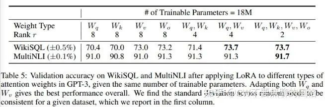
From the table, it can be seen that the model prefers us to apply LoRA to more types of projection matrices (as shown in the table, applying LoRA to all four projection matrices yields the best results), even though the rank is very low (as shown in the far-right column), which is sufficient for capturing enough information.
How to Implement It in Code
Assuming is a linear layer, let’s see how to implement LoRA on it.
(Please pay close attention to the comments in the code, thank you~)
class MergedLinear(nn.Linear, LoraLayer):
    # Lora implemented in a dense layer
    def __init__(
        self,
        in_features: int,
        out_features: int,
        r: int = 0,
        lora_alpha: int = 1,
        lora_dropout: float = 0.0,
        enable_lora: List[bool] = [False],
        fan_in_fan_out: bool = False,
        merge_weights: bool = True,
        **kwargs,
    ):
        nn.Linear.__init__(self, in_features, out_features, **kwargs)
        LoraLayer.__init__(self, r=r, lora_alpha=lora_alpha, lora_dropout=lora_dropout, merge_weights=merge_weights)

        # enable_lora is a boolean list indicating which "sub-parts" of the weight matrix should undergo low-rank decomposition.
        # For example, W is a matrix with shape (out_features, in_features),
        # then enable_lora = [True, False, True] means that W is divided into three parts W1, W2, W3 along the out_features dimension,
        # each having shape (out_features // 3, in_features), and only W1 and W3 undergo low-rank decomposition.
        # Here, W1's first dimension is in the range [0, out_features // 3), W3 is [2 * out_features // 3, out_features).
        # Similarly, if enable_lora = [True], it indicates that the entire W undergoes low-rank decomposition.
        if out_features % len(enable_lora) != 0:
            raise ValueError("The length of enable_lora must divide out_features")

        self.enable_lora = enable_lora
        self.fan_in_fan_out = fan_in_fan_out

        # Actual trainable parameters
        if r > 0 and any(enable_lora):
            # Only the parts where enable_lora = True apply low-rank decomposition, each part's low-rank is r
            self.lora_A = nn.Linear(in_features, r * sum(enable_lora), bias=False)
            # Note that here B is implemented using 1D grouped convolutions
            self.lora_B = nn.Conv1d(
                r * sum(enable_lora),
                out_features // len(enable_lora) * sum(enable_lora),
                kernel_size=1,
                groups=2,
                bias=False,
            )

            # Scale factor, scaling the output of the low-rank matrix (BAx)
            self.scaling = self.lora_alpha / self.r
            # Freezing the pre-trained weight matrix
            # Fixing the pre-trained weights
            self.weight.requires_grad = False

            # Compute the indices
            # Record which "sub-matrices" of the weight matrix underwent low-rank decomposition
            self.lora_ind = self.weight.new_zeros((out_features,), dtype=torch.bool).view(len(enable_lora), -1)
            self.lora_ind[enable_lora, :] = True
            self.lora_ind = self.lora_ind.view(-1)

        self.reset_parameters()
        if fan_in_fan_out:
            # fan_in_fan_out is for the Conv1D module of GPT-2,
            # which differs from Linear in that the dimensions are transposed
            self.weight.data = self.weight.data.T

    def reset_parameters(self):
        nn.Linear.reset_parameters(self)
        if hasattr(self, "lora_A"):
            # initialize A the same way as the default for nn.Linear and B to zero
            nn.init.kaiming_uniform_(self.lora_A.weight, a=math.sqrt(5))
            nn.init.zeros_(self.lora_B.weight)
The above class is called MergedLinear, and as the name suggests, it merges the low-rank decomposition part into the original pre-trained weights.
In the above code, the more complex part relates to the enable_lora parameter, which flexibly specifies which parts of the pre-trained weights should undergo low-rank decomposition.
Regarding the design of this parameter, I suspect this is because in some model implementations, the projection matrices in the Attention layers are implemented using a shared linear layer (like GPT-2, BLOOM, etc.), and with this enable_lora parameter, one can flexibly specify which of these three to undergo low-rank decomposition.
All layers that require low-rank decomposition will inherit from LoraLayer, which doesn’t have anything special; it just sets some properties that LoRA should have:
class LoraLayer:
    def __init__(
        self,
        r: int,
        lora_alpha: int,
        lora_dropout: float,
        merge_weights: bool,
    ):
        self.r = r
        self.lora_alpha = lora_alpha

        # Optional dropout
        if lora_dropout > 0.0:
            self.lora_dropout = nn.Dropout(p=lora_dropout)
        else:
            self.lora_dropout = lambda x: x

        # Mark the weight as unmerged
        # Mark whether the low-rank decomposition part has been merged into the pre-trained weights
        self.merged = False
        # Specify whether to merge the low-rank decomposition part into the pre-trained weights
        self.merge_weights = merge_weights

        # Whether to disable the low-rank decomposition part, if so, only use the pre-trained weights
        self.disable_adapters = False
Now, let’s introduce the forward process of the MergedLinear layer:
-
First, use the pre-trained weights to perform the forward process on the input to obtain ; -
Then feed the input into the low-rank decomposition matrix , obtaining the output ; -
Next, perform “zero-padding” on this part to match the shape of , and scale it; -
Finally, add this part back to , as shown in the formula.
def forward(self, x: torch.Tensor):
    result = F.linear(x, transpose(self.weight, self.fan_in_fan_out), bias=self.bias)
    if self.r > 0:
        after_A = self.lora_A(self.lora_dropout(x))
        after_B = self.lora_B(after_A.transpose(-2, -1)).transpose(-2, -1)
        result += self.zero_pad(after_B) * self.scaling

        return result
In point 3, the “zero-padding” corresponds to the zero_pad() in the above code. Earlier, CW mentioned the enable_lora parameter, which indicates that not all parts of the pre-trained weight matrix undergo low-rank decomposition, so the shape of the former may not be equal to that of the latter, hence it requires padding to allow both to perform element-wise addition.
Now let’s show the logic for this padding:
    def zero_pad(self, x):
        """ Zero-fill the output of the low-rank matrix BAx to align with the output Wx of the original weight matrix """
        result = x.new_zeros((*x.shape[:-1], self.out_features))
        result = result.view(-1, self.out_features)
        # Place BAx "in the right position" corresponding to Wx
        result[:, self.lora_ind] = x.reshape(-1, self.out_features // len(self.enable_lora) * sum(self.enable_lora))

        return result.view((*x.shape[:-1], self.out_features))
How to Achieve No Inference Delay
CW mentioned earlier that one of LoRA’s advantages is no inference delay (compared to the pre-trained model) because the low-rank decomposition part can be merged into the original pre-trained weights. For instance, when the model needs to infer, you would first call model.eval(), which is equivalent to calling model.train(mode=False), and then merge the low-rank decomposition part into the pre-trained weights as follows:
    def train(self, mode: bool = True):
        nn.Linear.train(self, mode)
        self.lora_A.train(mode)
        self.lora_B.train(mode)

        # Note: When calling model.eval(), train(mode=False) will be invoked
        # Merge the low-rank matrices A and B into the original weight matrix W
        if not mode and self.merge_weights and not self.merged:
            # Merge the weights and mark it
            if self.r > 0 and any(self.enable_lora):
                # \delta_W = BA
                delta_w = (
                    # Here, 1D convolution merges the low-rank matrices A and B:
                    # A(r * k) acts as input, r is treated as its channel, k is the spatial dimension size;
                    # B(d * r * 1) acts as convolution weights, d is the output channel, r is the input channel, 1 is the kernel size (note B is implemented as a 1D grouped convolution).
                    # Since it's a convolution, the 2D A needs to add a dimension for mini-batch: r * k -> 1 * r * k.
                    # After convolution, input (1 * r * k) -> output (1 * d * k)
                    F.conv1d(
                        self.lora_A.weight.data.unsqueeze(0),
                        self.lora_B.weight.data,
                        groups=sum(self.enable_lora),
                    )
                    .squeeze(0)  # 1 * d * k -> d * k
                    .transpose(-2, -1)  # d * k -> k * d
                )
                # zero_pad() is for zero-padding the low-rank decomposition matrix \delta_W, as some parts of the original weight matrix W may not have undergone low-rank decomposition,
                # to obtain a result aligned with the shape of the original weight matrix W, allowing for addition.
                # For the original weight matrix W being a Linear layer, fan_in_fan_out = False, thus this will require transpose: k * d -> D * k;
                # For the case where the original weight matrix W is the Conv1D of GPT-2, fan_in_fan_out=True, no transpose is needed, its out features are placed in the second dimension.
                # W = W + \delta_W
                self.weight.data += transpose(self.zero_pad(delta_w * self.scaling), not self.fan_in_fan_out)
        elif xxx:
            ...
Once merged, the forward process can proceed directly without needing to perform the steps as shown in the previous section:
def forward(self, x: torch.Tensor):
    # This part is omitted for now, will be introduced in the next section
    if xxx:
        ...
    # Low-rank decomposition part has been merged
    elif self.merged:
        return F.linear(x, transpose(self.weight, self.fan_in_fan_out), bias=self.bias)
    # Low-rank decomposition part has not been merged
    else:
        result = F.linear(x, transpose(self.weight, self.fan_in_fan_out), bias=self.bias)
        if self.r > 0:
            after_A = self.lora_A(self.lora_dropout(x))
            after_B = self.lora_B(after_A.transpose(-2, -1)).transpose(-2, -1)
            result += self.zero_pad(after_B) * self.scaling

        return result
How to Flexibly Switch in Downstream Tasks
Another attractive aspect of LoRA is that after fine-tuning the model on a certain downstream task A, the parameters of the low-rank matrices can be decoupled, restoring the pre-trained weights, allowing for continued fine-tuning on another downstream task B.
    def train(self, mode: bool = True):
        nn.Linear.train(self, mode)
        self.lora_A.train(mode)
        self.lora_B.train(mode)

        if xxx:
            ...
        # The previous branch represents mode=False, entering this branch indicates mode=True, i.e., calling model.train(),
        # When the low-rank matrices A and B have already been merged into the original weight matrix W,
        # they need to be decomposed to allow training (the pre-trained weight W does not need training).
        elif self.merge_weights and self.merged:
            # Make sure that the weights are not merged
            if self.r > 0 and any(self.enable_lora):
                # \delta_W = BA
                delta_w = (
                    F.conv1d(
                        self.lora_A.weight.data.unsqueeze(0),
                        self.lora_B.weight.data,
                        groups=sum(self.enable_lora),
                    )
                    .squeeze(0)
                    .transpose(-2, -1)
                )
                # W = W - \delta_W
                self.weight.data -= transpose(self.zero_pad(delta_w * self.scaling), not self.fan_in_fan_out)
            self.merged = False
After restoring the pre-trained weights, if you don’t want to use the parameters of the low-rank matrices, you can do so (see the following first branch):
    def forward(self, x: torch.Tensor):
        # When specifying not to use the adapters part (in this case, the low-rank decomposition matrix \delta_W=BA),
        # then the \delta_W that has been merged into the original weight W is decoupled, using only the pre-trained weight W for the forward operation on input x.
        if self.disable_adapters:
            if self.r > 0 and self.merged and any(self.enable_lora):
                delta_w = (
                    F.conv1d(
                        self.lora_A.weight.data.unsqueeze(0),
                        self.lora_B.weight.data,
                        groups=sum(self.enable_lora),
                    )
                    .squeeze(0)
                    .transpose(-2, -1)
                )
                # W = W - \delta_W
                self.weight.data -= transpose(self.zero_pad(delta_w * self.scaling), not self.fan_in_fan_out)
                self.merged = False
            return F.linear(x, transpose(self.weight, self.fan_in_fan_out), bias=self.bias)
        # When using adapters and the low-rank decomposition matrix \delta_W=BA has been merged into the pre-trained weight W, the forward process can proceed directly.
        elif self.merged:
            ...
        # When using adapters but the low-rank decomposition matrix \delta_W=BA has not been merged into the pre-trained weight W, the forward process is carried out in "steps":
        # First, use the pre-trained weight W to perform the forward process on the input x to obtain Wx;
        # Then feed the input x into the low-rank decomposition matrix \delta_W=BA to obtain the output of the adapters (\delta_W)x;
        # Next, perform zero-padding on the output of the adapters to match the shape of Wx, and scale it;
        # Finally, add this part back to Wx.
        else:
            ...
The Advancing LoRA
After tackling the seven questions about LoRA, it’s time for some deeper thinking.
Setting the Rank r
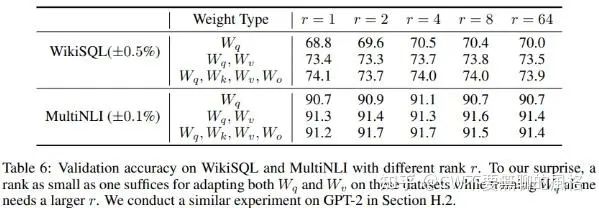
A direct question is: how should the rank r be set in practice?
The authors conducted several experiments for comparison and found that the rank can be very low, and setting it to no more than 8 is quite okay, even setting it to 1 works well.
Effectiveness of Low Rank
Seeing this experimental phenomenon, the author “couldn’t help” but think: having a very low intrinsic rank, increasing r does not allow it to cover more meaningful subspaces, long live low rank!
However, he is not just talking; he carefully conducted an experiment to verify this intuition. The specific approach was to use the same pre-trained model and apply LoRA with both and rank settings for fine-tuning, then extract the trained low-rank matrices and perform singular value decomposition to compare the overlap of the subspaces spanned by their top singular value vectors (using Grassmann Distance as a metric), as shown in the formula in the paper:
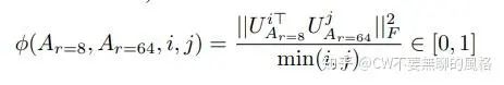
Where corresponds to the top-i singular value vectors of , and similarly. The range of is , the larger it is, the higher the overlap degree of the two subspaces.
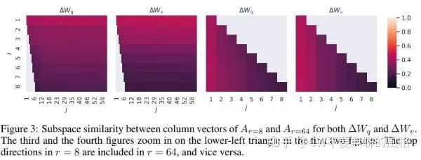
The experimental results shown in the figure indicate that the overlap of the spaces spanned by the top singular value vectors of both is highest, especially at the top-1, which also provides an explanation for the previous section’s “effectiveness”.
Since both settings used the same pre-trained model and underwent the same downstream training, the directions of the top singular value vectors are quite consistent (the rest of the directions are less correlated), indicating that the directions indicated by the top singular value vectors are the most useful for downstream task i, while other directions may be more random noise directions, which may have been accumulated during training.
Thus, low rank is indeed the correct answer.
Relationship Between Low-Rank Matrices and Pre-Trained Weight Matrices
When I first encountered LoRA, CW was curious about whether the trained matrices have any “blood relationship” with the original pre-trained weights, and how are they correlated?
The authors also explored this question. They mapped the to the r-dimensional subspace of , obtaining , where and are the left and right singular vector matrices respectively. They then calculated the Frobenius norm of . As a control group, the authors also mapped to its own and a random matrix’s top-r singular value vector space.
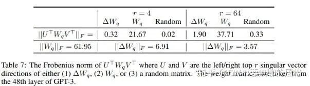
The experimental results indicate that the pre-trained weight matrix and the low-rank matrix are still “close relatives”: compared to the random matrix, the values after mapping to the subspace are higher.
Optimization Direction of Low-Rank Matrices
The above experimental results reveal two points:
-
Low-rank matrices amplify those vector directions that were not emphasized during pre-training; -
For the previous point, the amplification effect is stronger when r is low (
At first glance, the experimental results may not be easy to understand, so how should we interpret the first point?
We need to look back at the experiment result figure above. Regardless of whether it is or case, the Frobenius norms after mapping to the r-dimensional subspace are very small (0.32 & 1.90), indicating that the vector directions in these subspaces are not the high-priority directions in , but rather directions that were not emphasized during pre-training. However, it can be seen that is not so small (6.91 & 3.57), indicating that those originally less prominent directions have been emphasized.
Thus, it can be concluded that during the downstream training process, the low-rank matrices do not simply repeat the directions of the top singular value vectors of the pre-trained weight matrix, but instead amplify the directions that were not emphasized during pre-training.
As for the second point, we calculated the for both and cases, where takes the value of that column, and this calculation result measures the amplification effect of the low-rank matrices in the second point. Through computation, we can find that the amplification effect is stronger when the rank is relatively low, so what does this mean?
We have reason to believe that the low-rank matrix contains most of the vector directions relevant to downstream tasks (after all, it is optimized towards the best direction for downstream), thus the above calculation results indicate that the intrinsic rank of the matrix for adapting to downstream tasks is low.
Coincidentally! We have inadvertently proved again that low rank is indeed the right answer.
Is Low Rank Universally Applicable?
CW has repeatedly claimed that “low rank is the correct answer” is somewhat exaggerated. Firstly, the author’s experimental scenarios are quite limited and have not been verified across a broader range of cases; secondly, we should not blindly assume that a very small value of r will work in all tasks and datasets.
Imagine that when there is a huge difference (gap) between the downstream task and the pre-training task (for example, pre-training in English and fine-tuning in Chinese), using a small value of r is unlikely to yield good results. In this case, fine-tuning all model parameters (allowing r to be ) should yield better results, as the overlap of vector spaces between English and Chinese should not be very high, and we need to turn more parameters to adapt to the Chinese space.
Example: Fine-tuning BLOOM-7B with Around 12G of Memory on a Single Card
Finally, this section provides an example of fine-tuning using LoRA, based on Huggingface’s PEFT library, utilizing LoRA + 8bit training, where 8bit training requires the installation of bitsandbytes. With around 12G of memory on a single card, you can work with the 7B BLOOM model.
Some Tidbits
First, let’s handle some trivial matters: importing modules, setting dataset-related parameters, training parameters, and random seeds, etc.
import gc
import os
import sys
import psutil
import argparse
import threading

import torch
import torch.nn as nn

import numpy as np

from tqdm import tqdm

from torch.utils.data import DataLoader

from datasets import load_dataset
from accelerate import Accelerator
from transformers import (
    AutoModelForCausalLM,
    AutoTokenizer,
    default_data_collator,
    get_linear_schedule_with_warmup,
    set_seed,
)

from peft import LoraConfig, TaskType, get_peft_model, prepare_model_for_int8_training


def set_seed(seed: int):
    """
    Helper function for reproducible behavior to set the seed in `random`, `numpy`, `torch` and/or `tf` (if installed).

    Args:
        seed (`int`): The seed to set.
    """

    random.seed(seed)
    np.random.seed(seed)

    if is_torch_available():
        torch.manual_seed(seed)
        torch.cuda.manual_seed_all(seed)
        # ^^ safe to call this function even if cuda is not available

    if is_tf_available():
        tf.random.set_seed(seed)


def main():
    accelerator = Accelerator()

    dataset_name = "twitter_complaints"
    text_column = "Tweet text"
    label_column = "text_label"

    # The maximum sentence length of samples
    max_length = 64

    lr = 1e-3
    batch_size = 8
    num_epochs = 20

    # Set random seed (42 yyds!)
    seed = 42
    set_seed(seed)
Data Loading and Preprocessing
The dataset used here is RAFT (The Real-world Annotated Few-shot Tasks) task’s Twitter Complaints, which has 50 training samples and 3399 testing samples.
Below is the logic for data loading and preprocessing, the code itself is straightforward, no need for excessive explanation.
''' Datset and Dataloader '''

    dataset = load_dataset("ought/raft", dataset_name, cache_dir=args.data_cache_dir)
    classes = [k.replace("_", " ") for k in dataset["train"].features["Label"].names]
    dataset = dataset.map(
        lambda x: {"text_label": [classes[label] for label in x["Label"]]},
        batched=True,
        num_proc=4
    )

    # Preprocessing

    tokenizer = AutoTokenizer.from_pretrained(args.model_name_or_path, cache_dir=args.model_cache_dir)

    def preprocess_function(examples):
        # Note: The batch size here is not the same as the training batch size,
        # during this data preprocessing, it is also batch processing, so there is also a concept of batch size
        batch_size = len(examples[text_column])

        # Add prompt 'Label' to input text
        inputs = [f"{text_column} : {x} Label : " for x in examples[text_column]]
        targets = [str(x) for x in examples[label_column]]

        model_inputs = tokenizer(inputs)
        labels = tokenizer(targets)

        # Process each sample sequentially
        for i in range(batch_size):
            sample_input_ids = model_inputs["input_ids"][i]
            label_input_ids = labels["input_ids"][i] + [tokenizer.pad_token_id]

            # Align input text (model_inputs) with labels (labels), then set the corresponding input text part of the labels to -100,
            # so that during loss calculation, this part won't be counted, only the actual label text part will be calculated.
            # Add label text to input text
            model_inputs["input_ids"][i] = sample_input_ids + label_input_ids
            # Let the label value which corresponds to the input text word to be -100
            labels["input_ids"][i] = [-100] * len(sample_input_ids) + label_input_ids
            model_inputs["attention_mask"][i] = [1] * len(model_inputs["input_ids"][i])

        # Put pad tokens at the front of the inputs, and truncate to 'max_length'
        for i in range(batch_size):
            sample_input_ids = model_inputs["input_ids"][i]
            label_input_ids = labels["input_ids"][i]

            pad_length = max_length - len(sample_input_ids)
            labels["input_ids"][i] = [-100] * pad_length + label_input_ids
            model_inputs["input_ids"][i] = [tokenizer.pad_token_id] * pad_length + sample_input_ids
            model_inputs["attention_mask"][i] = [0] * pad_length + model_inputs["attention_mask"][i]

            # To tensor
            model_inputs["input_ids"][i] = torch.tensor(model_inputs["input_ids"][i][:max_length])
            model_inputs["attention_mask"][i] = torch.tensor(model_inputs["attention_mask"][i][:max_length])
            labels["input_ids"][i] = torch.tensor(labels["input_ids"][i][:max_length])

        model_inputs["labels"] = labels["input_ids"]
        return model_inputs

    def test_preprocess_function(examples):
        batch_size = len(examples[text_column])

        inputs = [f"{text_column} : {x} Label : " for x in examples[text_column]]
        model_inputs = tokenizer(inputs)

        for i in range(batch_size):
            sample_input_ids = model_inputs["input_ids"][i]

            pad_length = max_length - len(sample_input_ids)
            model_inputs["input_ids"][i] = [tokenizer.pad_token_id] * pad_length + sample_input_ids
            model_inputs["attention_mask"][i] = [0] * pad_length + model_inputs["attention_mask"][i]

            # To tensor
            model_inputs["input_ids"][i] = torch.tensor(model_inputs["input_ids"][i][:max_length])
            model_inputs["attention_mask"][i] = torch.tensor(model_inputs["attention_mask"][i][:max_length])

        return model_inputs

    with accelerator.main_process_first():
        processed_datasets = dataset.map(
            preprocess_function,
            batched=True,
            num_proc=4,
            remove_columns=dataset["train"].column_names,
            load_from_cache_file=True,
            desc="Running tokenizer on dataset",
        )
    accelerator.wait_for_everyone()
    train_dataset = processed_datasets["train"]

    with accelerator.main_process_first():
        processed_datasets = dataset.map(
            test_preprocess_function,
            batched=True,
            num_proc=4,
            remove_columns=dataset["train"].column_names,
            load_from_cache_file=False,
            desc="Running tokenizer on dataset",
        )
    eval_dataset = processed_datasets["train"]
    test_dataset = processed_datasets["test"]

    # Dataloaders
    train_dataloader = DataLoader(
        train_dataset, shuffle=True, collate_fn=default_data_collator,
        batch_size=batch_size, pin_memory=True, num_workers=4
    )
    eval_dataloader = DataLoader(
        eval_dataset, collate_fn=default_data_collator,
        batch_size=batch_size, pin_memory=True, num_workers=4
    )
    test_dataloader = DataLoader(
        test_dataset, collate_fn=default_data_collator,
        batch_size=batch_size, pin_memory=True, num_workers=4
    )

    print(f"The 1st train batch sample: {next(iter(train_dataloader))}\n")
Model, Optimizer & Lr Scheduler
Essentials: model, optimizer, learning rate scheduling.
''' Model, Optimizer, Lr Scheduler '''

    # creating model
    model = AutoModelForCausalLM.from_pretrained(
        args.model_name_or_path,
        cache_dir=args.model_cache_dir,
        load_in_8bit=args.load_in_8bit,
        device_map='auto'  # A device map needs to be passed to run convert models into mixed-int8 format
    )

    ''' Post-processing on the model, includes:
        1- Cast the layernorm in fp32;
        2- making output embedding layer require grads;
        3- Anable gradient checkpointing for memory efficiency;
        4- Add the upcasting of the lm head to fp32
    '''
    model = prepare_model_for_int8_training(model)

    # Configure some parameters for LoRA
    peft_config = LoraConfig(task_type=TaskType.CAUSAL_LM, inference_mode=False, r=8, lora_alpha=32, lora_dropout=0.1)
    # Apply LoRA to the model
    model = get_peft_model(model, peft_config)

    # Print the number of trainable parameters
    model.print_trainable_parameters()

    # optimizer
    optimizer = torch.optim.AdamW(model.parameters(), lr=args.lr)

    # lr scheduler
    lr_scheduler = get_linear_schedule_with_warmup(
        optimizer=optimizer,
        num_warmup_steps=0,
        num_training_steps=(len(train_dataloader) * num_epochs),
    )

    model, train_dataloader, eval_dataloader, test_dataloader, optimizer, lr_scheduler = accelerator.prepare(
        model, train_dataloader, eval_dataloader, test_dataloader, optimizer, lr_scheduler
    )
    accelerator.print(f"Model: {model}\n")
Preparation for 8bit Training
This section further explains the model = prepare_model_for_int8_training(model) part from the previous section, which is aimed at stabilizing the training process for better results. Let’s see what it specifically does.
def prepare_model_for_int8_training(
    model, output_embedding_layer_name="lm_head", use_gradient_checkpointing=True, layer_norm_names=["layer_norm"]
):
    r"""
    This method wraps the entire protocol for preparing a model before running a training. This includes:
        1- Cast the layernorm in fp32 2- making output embedding layer require grads 3- Add the upcasting of the lm
        head to fp32

    Args:
        model, (`transformers.PreTrainedModel`):
            The loaded model from `transformers`
    """
    loaded_in_8bit = getattr(model, "is_loaded_in_8bit", False)

    # 1. Fix the pre-trained weights;
    # 2. Convert the Layer Norm parameters to fp32 for training stability
    for name, param in model.named_parameters():
        # freeze base model's layers
        param.requires_grad = False

        if loaded_in_8bit:
            # cast layer norm in fp32 for stability for 8bit models
            if param.ndim == 1 and any(layer_norm_name in name for layer_norm_name in layer_norm_names):
                param.data = param.data.to(torch.float32)

    # Allow the Embedding layer to accept gradients, achieved by registering a forward hook on the Embedding layer,
    # the forward hook's content will be called after the model's forward process completes.
    # The hook's content is to ensure that the output of the Embedding layer accepts gradients,
    # allowing the gradients to propagate to the Embedding layer.
    if loaded_in_8bit and use_gradient_checkpointing:
        # For backward compatibility
        if hasattr(model, "enable_input_require_grads"):
            model.enable_input_require_grads()
        else:

            def make_inputs_require_grad(module, input, output):
                output.requires_grad_(True)

            model.get_input_embeddings().register_forward_hook(make_inputs_require_grad)

        # Enable gradient checkpointing for memory efficiency
        # Optimize the gradients of the intermediate activations during the forward process to optimize memory usage.
        model.gradient_checkpointing_enable()

    # Convert the output of the model's head to fp32 for stable training
    if hasattr(model, output_embedding_layer_name):
        output_embedding_layer = getattr(model, output_embedding_layer_name)
        input_dtype = output_embedding_layer.weight.dtype

        class CastOutputToFloat(torch.nn.Sequential):
            r"""
            Manually cast to the expected dtype of the lm_head as sometimes there is a final layer norm that is casted
            in fp32

            """
            def forward(self, x):
                # The reason for converting the input (x) to the expected dtype of this layer's parameters is that the previous layer may be Layer Norm,
                # as we know, we converted the precision of Layer Norm's output to fp32, so in this case, we need to convert the output (the input of this layer) to the same precision as this layer's parameters.
                return super().forward(x.to(input_dtype)).to(torch.float32)

        setattr(model, output_embedding_layer_name, CastOutputToFloat(output_embedding_layer))

    return model
From the above source code implementation and CW’s comments, we can see that this part mainly does the following four things:
-
Convert the parameters of LayerNorm to fp32; -
Allow the Embedding layer’s output to accept gradients, thus enabling the gradients to propagate to that layer; -
Optimize the gradients of the intermediate activations generated during the forward process to reduce memory consumption; -
Convert the output precision of the model head (Head) to fp32.
PEFT Model
In this section, CW will lead everyone to see how to convert a regular model to a PEFT model: _model = get_peft_model(model, peft_config)_ for the case of the BLOOM model.
def get_peft_model(model, peft_config):
    """
    Returns a Peft model object from a model and a config.

    Args:
        model ([`transformers.PreTrainedModel`]): Model to be wrapped.
        peft_config ([`PeftConfig`]): Configuration object containing the parameters of the Peft model.
    """

    model_config = model.config.to_dict()
    peft_config.base_model_name_or_path = model.__dict__.get("name_or_path", None)

    if peft_config.task_type not in MODEL_TYPE_TO_PEFT_MODEL_MAPPING.keys():
        peft_config = _prepare_lora_config(peft_config, model_config)
        return PeftModel(model, peft_config)

    if not isinstance(peft_config, PromptLearningConfig):
        # BLOOM will enter this branch
        peft_config = _prepare_lora_config(peft_config, model_config)
    else:
        peft_config = _prepare_prompt_learning_config(peft_config, model_config)

    # In our example, peft_config.task_type is CAUSAL_LM,
    # MODEL_TYPE_TO_PEFT_MODEL_MAPPING[peft_config.task_type] is PeftModelForCausalLM,
    # which is a subclass of PeftModel that is the result of applying LoRA transformations to the target module of the original model
    return MODEL_TYPE_TO_PEFT_MODEL_MAPPING[peft_config.task_type](model, peft_config)
Let’s further look at the implementation of peft_config = _prepare_lora_config(peft_config, model_config), which determines which modules of the model will apply LoRA.
def _prepare_lora_config(peft_config, model_config):
    if peft_config.target_modules is None:
        if model_config["model_type"] not in TRANSFORMERS_MODELS_TO_LORA_TARGET_MODULES_MAPPING:
            raise ValueError("Please specify `target_modules` in `peft_config`")
        # Set the target modules for LoRA transformation, usually one or several mapping matrices in the Attention layers
        # For BLOOM, this returns ["query_key_value"], corresponding to the QKV mapping matrices in the BloomAttention implementation
        peft_config.target_modules = TRANSFORMERS_MODELS_TO_LORA_TARGET_MODULES_MAPPING[model_config["model_type"]]

    if len(peft_config.target_modules) == 1:
        # This is only valid for Conv1D used in GPT-2
        peft_config.fan_in_fan_out = True
        # These three values represent whether to apply LoRA to the Q, K, V mapping matrices
        # For BLOOM, only the Q and V mapping matrices undergo transformation, while K does not.
        peft_config.enable_lora = [True, False, True]

    if peft_config.inference_mode:
        # If in inference mode, the low-rank matrices A and B will be merged into the original weight matrix W
        peft_config.merge_weights = True

    return peft_config
Combining CW’s comments in the code above, we can see that for BLOOM, peft_config.target_modules is [“query_key_value”], which corresponds to the Q, K, V mapping matrices in its submodule BloomAttention:
class BloomAttention(nn.Module):
    def __init__(self, config: BloomConfig):
        super().__init__()

        # Omitted parts
        ...

        self.hidden_size = config.hidden_size
        self.num_heads = config.n_head
        self.head_dim = self.hidden_size // self.num_heads
        self.split_size = self.hidden_size
        self.hidden_dropout = config.hidden_dropout

        # Omitted parts
        ...

        # ["query_key_value"] refers to this module
        self.query_key_value = nn.Linear(self.hidden_size, 3 * self.hidden_size, bias=True)
        self.dense = nn.Linear(self.hidden_size, self.hidden_size)
        self.attention_dropout = nn.Dropout(config.attention_dropout)
This target_modules also supports customization as long as it matches the keywords in the model implementation.
Training
Training is essentially a conventional iterative process, but the highlight here is the use of the TorchTracemalloc context manager, which conveniently calculates the consumption of GPU and CPU (in MB).
    for epoch in range(num_epochs):
        with TorchTracemalloc() as tracemalloc:
            model.train()

            total_loss = 0
            for step, batch in enumerate(tqdm(train_dataloader)):
                # Forward
                outputs = model(**batch)
                loss = outputs.loss
                total_loss += loss.detach().float()

                # Backward
                accelerator.backward(loss)
                optimizer.step()
                lr_scheduler.step()

                optimizer.zero_grad()

                if step % 3 == 0:
                    accelerator.print(f"epoch {epoch + 1}\t step {step + 1}\t loss {loss.item()}")
            epoch_loss = total_loss / len(train_dataloader)
            epoch_ppl = torch.exp(epoch_loss)
            accelerator.print(f"[Epoch{epoch + 1}]\t total loss: {epoch_loss}\t perplexity: {epoch_ppl}\n")

        # Printing the GPU memory usage details such as allocated memory, peak memory, and total memory usage
        accelerator.print("GPU Memory before entering the train : {}".format(b2mb(tracemalloc.begin)))
        accelerator.print("GPU Memory consumed at the end of the train (end-begin): {}".format(tracemalloc.used))
        accelerator.print("GPU Peak Memory consumed during the train (max-begin): {}".format(tracemalloc.peaked))
        accelerator.print(
            "GPU Total Peak Memory consumed during the train (max): {}\n".format(
                tracemalloc.peaked + b2mb(tracemalloc.begin)
            )
        )

        accelerator.print("CPU Memory before entering the train : {}".format(b2mb(tracemalloc.cpu_begin)))
        accelerator.print("CPU Memory consumed at the end of the train (end-begin): {}".format(tracemalloc.cpu_used))
        accelerator.print("CPU Peak Memory consumed during the train (max-begin): {}".format(tracemalloc.cpu_peaked))
        accelerator.print(
            "CPU Total Peak Memory consumed during the train (max): {}\n".format(
                tracemalloc.cpu_peaked + b2mb(tracemalloc.cpu_begin)
            )
        )

        train_epoch_loss = total_loss / len(eval_dataloader)
        train_ppl = torch.exp(train_epoch_loss)
        accelerator.print(f"{epoch=}: {train_ppl=} {train_epoch_loss=}\n")
By the way, here’s a showcase of GPU and CPU resource consumption during training (all units are in MB):
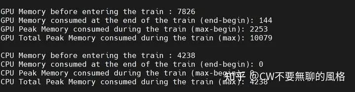
Resource consumption during training for a certain epoch
Oh? You say you’re curious about how TorchTracemalloc works? OK, CW won’t hold back, here you go:
def b2mb(x):
    """ Converting Bytes to Megabytes. """
    return int(x / 2**20)


class TorchTracemalloc:
    """ This context manager is used to track the peak memory usage of the process. """

    def __enter__(self):
        gc.collect()
        torch.cuda.empty_cache()
        # Reset the peak gauge to zero
        torch.cuda.reset_max_memory_allocated()

        # Return current memory usage
        self.begin = torch.cuda.memory_allocated()
        self.process = psutil.Process()

        self.cpu_begin = self.cpu_mem_used()

        self.peak_monitoring = True
        peak_monitor_thread = threading.Thread(target=self.peak_monitor_func)
        peak_monitor_thread.daemon = True
        peak_monitor_thread.start()

        return self

    def cpu_mem_used(self):
        """Get resident set size memory for the current process"""
        return self.process.memory_info().rss

    def peak_monitor_func(self):
        self.cpu_peak = -1

        while True:
            self.cpu_peak = max(self.cpu_mem_used(), self.cpu_peak)

            # can't sleep or will not catch the peak right (this comment is here on purpose)
            # time.sleep(0.001) # 1msec

            if not self.peak_monitoring:
                break

    def __exit__(self, *exc):
        self.peak_monitoring = False

        gc.collect()
        torch.cuda.empty_cache()

        self.end = torch.cuda.memory_allocated()
        self.peak = torch.cuda.max_memory_allocated()

        self.used = b2mb(self.end - self.begin)
        self.peaked = b2mb(self.peak - self.begin)

        self.cpu_end = self.cpu_mem_used()
        self.cpu_used = b2mb(self.cpu_end - self.cpu_begin)
        self.cpu_peaked = b2mb(self.cpu_peak - self.cpu_begin)
Evaluation
Evaluation is similar to training, but the forward process needs to call the model’s generate() method rather than forward(), as the former is in an auto-regressive manner.
        model.eval()

        eval_preds = []
        with TorchTracemalloc() as tracemalloc:
            for batch in tqdm(eval_dataloader):
                batch = {k: v for k, v in batch.items() if k != "labels"}

                with torch.no_grad():
                    # Note: The inference process uses an auto-regressive manner, calling the model's generate() method
                    outputs = accelerator.unwrap_model(model).generate(**batch, max_new_tokens=10)
                outputs = accelerator.pad_across_processes(outputs, dim=1, pad_index=tokenizer.pad_token_id)

                preds = accelerator.gather(outputs)
                # The part before 'max_length' belongs to prompts
                preds = preds[:, max_length:].detach().cpu().numpy()
                # 'skip_special_tokens=True' will ignore those special tokens (e.g., pad token)
                eval_preds.extend(tokenizer.batch_decode(preds, skip_special_tokens=True))

        # Printing the GPU memory usage details such as allocated memory, peak memory, and total memory usage
        accelerator.print("GPU Memory before entering the eval : {}".format(b2mb(tracemalloc.begin)))
        accelerator.print("GPU Memory consumed at the end of the eval (end-begin): {}".format(tracemalloc.used))
        accelerator.print("GPU Peak Memory consumed during the eval (max-begin): {}".format(tracemalloc.peaked))
        accelerator.print(
            "GPU Total Peak Memory consumed during the eval (max): {}\n".format(
                tracemalloc.peaked + b2mb(tracemalloc.begin)
            )
        )

        accelerator.print("CPU Memory before entering the eval : {}".format(b2mb(tracemalloc.cpu_begin)))
        accelerator.print("CPU Memory consumed at the end of the eval (end-begin): {}".format(tracemalloc.cpu_used))
        accelerator.print("CPU Peak Memory consumed during the eval (max-begin): {}".format(tracemalloc.cpu_peaked))
        accelerator.print(
            "CPU Total Peak Memory consumed during the eval (max): {}\n".format(
                tracemalloc.cpu_peaked + b2mb(tracemalloc.cpu_begin)
            )
        )

        assert len(eval_preds) == len(dataset["train"][label_column]), \
            f"{len(eval_preds)} != {len(dataset['train'][label_column])}"

        correct = total = 0
        for pred, true in zip(eval_preds, dataset["train"][label_column]):
            if pred.strip() == true.strip():
                correct += 1
            total += 1

        accuracy = correct / total * 100
        accelerator.print(f"{accuracy=}\n")
        accelerator.print(f"Pred of the first 10 samples:\n {eval_preds[:10]=}\n")
        accelerator.print(f"Truth of the first 10 samples:\n {dataset["train"][label_column][:10]=}\n")
During inference, the GPU and CPU consumption is as follows (all units are in MB):
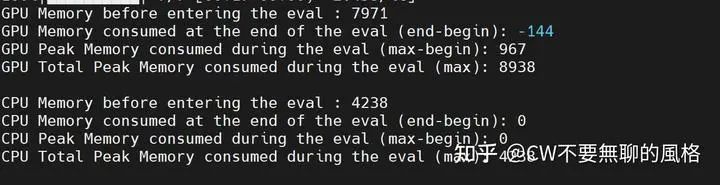
Resource consumption during inference after training for a certain epoch
End
As one of the hottest technologies in today’s large model era, whether LoRA counts as the right approach for fine-tuning LLMs is up to you to decide. More than correctness, suitability is what matters most. For me, I just think it’s fun rather than boring!