Introduction

With the continuous expansion of model scale, the feasibility of fine-tuning all parameters of the model (so-called full fine-tuning) is becoming increasingly low. Taking GPT-3 with 175 billion parameters as an example, each new domain requires a complete fine-tuning of a new model, which is very costly!

Paper: LORA: LOW-RANK ADAPTATION OF LARGE LANGUAGE MODELS^[1] Code: https://github.com/microsoft/LoRA

Problems with Existing Solutions

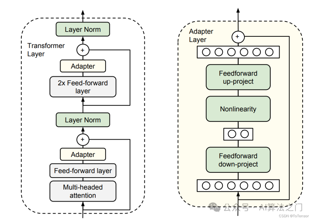
Adapter Tuning

In simple terms, an adapter fixes the original parameters and adds some extra parameters for fine-tuning. In the image above, two adapters will be added to the original transformer block, one after the multi-head attention and the other after the FFN.

As can be seen from the figure, the adapter increases the number of layers in the model, leading to slower inference speed.

Prefix Tuning

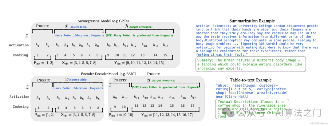
Specifically, for each layer in the transformer, a trainable virtual token embedding is inserted before the sentence representation. For autoregressive models (like the GPT series), a continuous prefix is added at the beginning of the sentence, i.e., Z = [PREFIX; x; y]. For Encoder-Decoder models (like T5), continuous prefixes are added before both the Encoder and Decoder: Z = [PREFIX; x | PREFIX; y]. The process of adding prefixes is shown in the figure above.

Although prefix-tuning does not add too many extra parameters, it is difficult to optimize and reduces the sequence length for downstream tasks.

LoRA

Several key advantages of LoRA:

• Pre-trained models can be shared, saving disk space• When switching tasks, only the LoRA weights need to be changed, which is cost-effective• During training, only the LoRA weights need to be trained, resulting in low memory consumption

Simply put: next to the model’s Linear layer, an “auxiliary” is added, which serves to replace the original parameter matrix W during training.

Combining with the above image, let’s intuitively understand this process. The input $x$, with dimension $d$, could be the output of embedding in a standard transformer model, or the output from the previous transformer layer, where $d$ is generally 768 (most BERT outputs have a dimension of 768). Following the original route, it should only go through the left side, which is the original model part.

However, under the LoRA strategy, an “auxiliary” on the right side is added, which first uses a Linear layer A to reduce the data from dimension $d$ to dimension $r$. This $r$ is the rank of LoRA, which is the most important hyperparameter in LoRA. It is usually much smaller than $d$ (commonly seen values are 4 or 8), especially for current large models where $d$ is often more than 768 or 1024; for example, in LLaMA-7B, each transformer layer has 32 heads, making $d$ reach 4096.

Next, a second Linear layer B is used to transform the data back from dimension $r$ to dimension $d$. Finally, the results from both sides are added together to obtain the output hidden_state.

For the two parts, the right side appears to be a decomposition of the original matrix $W$ on the left, reducing the number of parameters from $d * d$ to $d * r + r * d$, which is $2 * d * r$. When $r << d$, the number of parameters is significantly reduced.

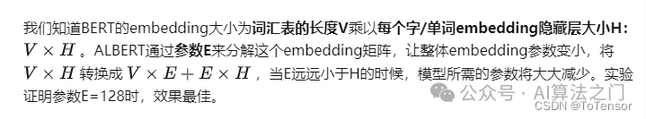
In Albert, the authors considered that the vocabulary dimension is large, so they decomposed the embedding matrix into two relatively smaller matrices to simulate the effect of the embedding matrix, thus greatly reducing the number of parameters to be trained (in fact, it reduced about 10M parameters, which is mainly due to cross-layer parameter sharing).

LoRA follows a similar idea and is not limited to the embedding layer; theoretically, it can be applied wherever large matrices appear.

However, unlike Albert, which directly replaces the original large matrix with two smaller matrices, LoRA retains the original matrix W but does not allow W to participate in training, so the parts that need to compute gradients are only the two smaller matrices A and B of the auxiliary.

From the equations in the paper, during full parameter fine-tuning, the model training optimization is expressed as (taking autoregressive language models as an example):

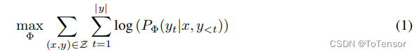
That is to maximize the conditional probability.

Where the model’s parameters are denoted by $\Phi$.

A major drawback of full parameter fine-tuning is that each downstream task requires learning a different set of parameters. If the pre-trained model is very large, such as GPT-3 (with 175 billion parameters), storing and deploying many independent fine-tuned model instances can be a challenge.

After adding LoRA, the model’s optimization is expressed as:

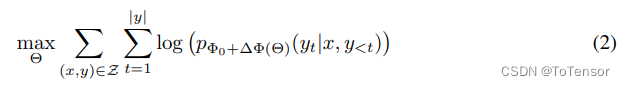
Where the original model parameters are $\\Phi_0$, and the new LoRA parameters are $\\Delta \\Phi(\Theta)$.

From the second equation, it can be seen that although the parameters appear to have increased (with $\\Delta \\Phi(\Theta)$ added), according to the previous max target, the parameters that need to be optimized are only $\Theta$, and according to the assumption, $\Theta << \Phi$, which greatly reduces the gradient computation during training. Thus, in low-resource situations, we can only consume resources from this part, allowing us to train large models under low memory conditions on a single card.

After training, only the parameters of the LoRA part (the trainable parameters) are saved. During inference, these parameters can be added to the original model to form a new model (the large ‘+’ part at the top of Figure 1), and then loaded for inference, which does not increase any additional inference time overhead compared to the original model.

Current LLMs are trained on hundreds of millions of data. LoRA, by maintaining the gradient of the original model, can avoid the collapse of the generalization ability of pre-training. This is because during the pre-training process, the model has learned a large amount of linguistic knowledge and structure, which can be applied to various downstream tasks. However, during complete fine-tuning, all parameters of the model are retrained, which may cause the model to forget previously learned knowledge and structure, thus reducing the model’s generalization ability.

In contrast, LoRA only fine-tunes a portion of the parameters while preserving the gradient of the original model. The advantage of this approach is that LoRA can fine-tune specific tasks while maintaining the language knowledge and structure of the original model, thereby improving the model’s performance. Additionally, the low-rank matrix injection method of LoRA can further enhance the model’s generalization ability because low-rank matrices can capture commonalities and patterns in the data, thus reducing the risk of overfitting.

Therefore, by preserving the gradient of the original model, LoRA can avoid the collapse of pre-training generalization ability and improve the generalization ability and performance of the model.

Official Implementation

Here, only the implementation of LoRA in the Linear layer is posted. For the full code, refer to: https://github.com/microsoft/LoRA

class Linear(nn.Linear, LoRALayer):    # LoRA implemented in a dense layer    def __init__(        self,         in_features: int,         out_features: int,         r: int = 0,         lora_alpha: int = 1,         lora_dropout: float = 0.,        fan_in_fan_out: bool = False, # Set this to True if the layer to replace stores weight like (fan_in, fan_out)        merge_weights: bool = True,        **kwargs    ):        nn.Linear.__init__(self, in_features, out_features, **kwargs)        LoRALayer.__init__(self, r=r, lora_alpha=lora_alpha, lora_dropout=lora_dropout,                           merge_weights=merge_weights)        self.fan_in_fan_out = fan_in_fan_out        # Actual trainable parameters        if r > 0:            self.lora_A = nn.Parameter(self.weight.new_zeros((r, in_features)))            self.lora_B = nn.Parameter(self.weight.new_zeros((out_features, r)))            self.scaling = self.lora_alpha / self.r            # Freezing the pre-trained weight matrix            self.weight.requires_grad = False        self.reset_parameters()        if fan_in_fan_out:            self.weight.data = self.weight.data.transpose(0, 1)    def reset_parameters(self):        nn.Linear.reset_parameters(self)        if hasattr(self, 'lora_A'):            # initialize A the same way as the default for nn.Linear and B to zero            nn.init.kaiming_uniform_(self.lora_A, a=math.sqrt(5))            nn.init.zeros_(self.lora_B)    def train(self, mode: bool = True):        def T(w):            return w.transpose(0, 1) if self.fan_in_fan_out else w        nn.Linear.train(self, mode)        if mode:            if self.merge_weights and self.merged:                # Make sure that the weights are not merged                if self.r > 0:                    self.weight.data -= T(self.lora_B @ self.lora_A) * self.scaling                self.merged = False        else:            if self.merge_weights and not self.merged:                # Merge the weights and mark it                if self.r > 0:                    self.weight.data += T(self.lora_B @ self.lora_A) * self.scaling                self.merged = True       def forward(self, x: torch.Tensor):        def T(w):            return w.transpose(0, 1) if self.fan_in_fan_out else w        if self.r > 0 and not self.merged:            result = F.linear(x, T(self.weight), bias=self.bias)            if self.r > 0:                result += (self.lora_dropout(x) @ self.lora_A.transpose(0, 1) @ self.lora_B.transpose(0, 1)) * self.scaling            return result        else:            return F.linear(x, T(self.weight), bias=self.bias

From the implementation code, it can also be seen that LoRA freezes the parameters of the PLM, and the actual parameters that need to be trained are only lora_A and lora_B. Moreover, during training, the PLM weights need to participate in the computation; therefore, LoRA is not efficient for training.

Conclusion

• LoRA is parameter-efficient but not training-efficient. The trainable parameters are indeed significantly reduced, but there is no obvious speed improvement in training on a single card. In LoRA, the entire PLM needs to participate in the backpropagation computation, not just the parts of the parameters in the bypass. This is because the low-rank matrix injection method of LoRA requires the gradient information from the entire PLM to calculate the gradient of the injected matrix. Specifically, the gradient calculation of LoRA includes two steps: first, the gradient of the entire PLM needs to be calculated; then, these gradients are used to calculate the gradient of the injected matrix.• In multi-card training, LoRA’s speed advantage is mainly reflected in two aspects: 1. Computational efficiency: Since LoRA only needs to compute and optimize the injected low-rank matrix, its computational efficiency is higher than that of full fine-tuning. In multi-card training, LoRA can distribute the computation and optimization of the injected matrix across multiple GPUs, thus accelerating the training process.2. Communication efficiency: In multi-card training, communication efficiency is often a bottleneck. Since LoRA only needs to communicate the parameters of the injected matrix, its communication efficiency is higher than that of full fine-tuning. In multi-card training, LoRA can distribute the parameters of the injected matrix across multiple GPUs, thus reducing communication volume and time. Therefore, LoRA is generally faster than full fine-tuning in multi-card training. Specifically, LoRA can reduce the hardware threshold by up to three times, thereby improving training efficiency.

References:

•Paper Reading: LORA – Low-Rank Adaptation of Large Language Models^[2]•Large Model Training – Introduction to PEFT and LoRA^[3]•Ladder Side-Tuning: The “Over-the-Wall” Ladder for Pre-trained Models^[4]

References

[1] LORA: LOW-RANK ADAPTATION OF LARGE LANGUAGE MODELS: https://arxiv.org/pdf/2106.09685.pdf[2] Paper Reading: LORA – Low-Rank Adaptation of Large Language Models: https://zhuanlan.zhihu.com/p/611557340[3] Large Model Training – Introduction to PEFT and LoRA: https://blog.csdn.net/weixin_44826203/article/details/129733930[4] Ladder Side-Tuning: The “Over-the-Wall” Ladder for Pre-trained Models: https://kexue.fm/archives/9138

To join the technical exchange group, please add the AINLP assistant on WeChat (id: ainlp2) and specify your specific direction and the relevant technical points used.