LoRA (Low-Rank Adaptation) is one of the parameter-efficient fine-tuning methods for current LLMs. Previously, we briefly discussed it in “LoRA from a Gradient Perspective: Introduction, Analysis, Speculation, and Promotion”. In this article, we will learn a new conclusion about LoRA:
Assigning different learning rates to the two matrices of LoRA can further enhance its performance.
This conclusion comes from the recent paper “LoRA+: Efficient Low-Rank Adaptation of Large Models”[1] (hereafter referred to as “LoRA+”). At first glance, this conclusion may not seem particularly special, because configuring different learning rates introduces a new hyperparameter, and generally speaking, introducing and fine-tuning hyperparameters often leads to improvements.
What is special about “LoRA+” is that it theoretically affirms this necessity and asserts that the optimal solution must have the learning rate of the right matrix greater than that of the left matrix. In short, “LoRA+” serves as a classic example of theory guiding training and proving effective in practice, worthy of careful study.
Conclusion Analysis
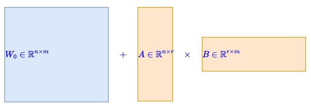
Assuming the pre-trained parameters are , if full parameter fine-tuning is used, then the increment is also a matrix. To reduce the number of parameters, LoRA constrains the update amount to a low-rank matrix, that is, set , where replaces the model’s original parameters, and then keeps unchanged, only updating A and B during training, as shown in the figure below:
Note that LoRA is usually applied to Dense layers, but the original paper’s analysis is based on weights multiplying inputs from the left, while implementations generally multiply inputs by weights from the right. To avoid confusion, this article aligns with the implementation notation, assuming the input of the layer is , and the operation of the layer is . Since the conclusion of “LoRA+” is independent of the pre-trained weights, we can generally set , simplifying the layer operation to .
The conclusion of “LoRA+” is: To make LoRA’s effect as close to optimal as possible, the learning rate of weight B should be greater than that of weight A.
Note that to make the initial model equivalent to the original pre-trained model, LoRA typically initializes one of A or B to all zeros. Initially, I thought this conclusion was due to the all-zero initialization, so it should depend on the position of the all-zero initialization, but after careful reading, I found that the conclusion claimed by “LoRA+” is unrelated to the all-zero initialization. In other words, although A and B appear symmetric, they inherently possess asymmetry such that regardless of whether A or B is initialized to all zeros, the conclusion remains that the learning rate of B must be greater than that of A. This is intriguing.It must be said that the derivation in the original paper of “LoRA+” is quite confusing. Below, I will attempt to complete the derivation using my own reasoning. Generally, it is based on two assumptions:1. Numerical Stability: The output values of each layer of the model should be numerically stable, independent of network width;2. Equivalent Contribution: To make LoRA optimal, the two matrices A and B should contribute equally to the performance.Next, we will analyze and quantify these two assumptions one by one.
Numerical Stability
First, numerical stability means that each component of X, XA, and XAB should be of the same order, independent of network widths n and m. Here, the primarily describes its order concerning network width, and does not imply that its absolute value is close to 1.This assumption should be uncontroversial; it is hard to imagine a numerically unstable network producing good predictive performance. However, some readers may question the necessity of “XA is “, because is the input and is the output, requiring their numerical stability makes sense, but must XA, as an intermediate variable, also be numerically stable?Looking at forward propagation alone, the numerical stability of XA is indeed not necessary. However, if XA is numerically unstable while XAB is numerically stable, then there are two scenarios: XA is numerically large, and B is numerically small, which will cause A’s gradient to be small and B’s gradient to be large according to the derivative formula; conversely, if XA is numerically small and B is numerically large, this will lead to A’s gradient being large and B’s gradient being small.In summary, the numerical instability of XA will lead to unstable gradients for A and B, thereby increasing optimization difficulty, so it is better to include the numerical stability of XA as a condition.This numerical stability condition easily reminds us of “LeCun Initialization”[2], which states that if Of course, as mentioned earlier, LoRA typically requires one of A or B to be initialized to all zeros to maintain the identity of the initialization, but this is not very important. We only need to recognize that a variance of 1/n and 1/r can keep XA and XAB numerically stable, which leads us to speculate that after training, A and B will likely also have variances close to 1/n and 1/r. Given that , this is equivalent to saying that the absolute value of A’s components will be significantly smaller than that of B’s components, which is the source of the asymmetry between A and B.
Equivalent Contribution
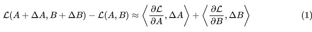
Next, let’s look at the second assumption: A and B should contribute equally to the performance. This assumption also seems reasonable, because in the scenario of LLM+LoRA, we usually have m=n, meaning A and B have the same number of parameters, making it reasonable for them to contribute equally to the performance. If we have , we can further generalize this assumption to say that the contribution to performance is proportional to the number of parameters. The most basic measure of performance is naturally the loss function, denoted as .We want to measure the change in the loss function when is modified:
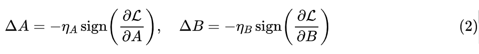
Here, a first-order linear approximation is used, where is the gradient of A and B, and is the (Frobenius) inner product operation. The right-hand side can be understood as the respective contributions of A and B to the performance. However, note that the validity of the linear approximation depends on the increment being small, but for well-trained weights, the increment relative to the original weights may not necessarily be small.Thus, we can relax our assumption of “equivalent contribution” to “A and B should contribute equally to the performance at each update step”, since the update amount at each step is usually small, the linear approximation can be reasonably satisfied.Since we need to consider the update amount at each step, this leads us to the direction of optimizers. Currently, the mainstream optimizers for pre-training and fine-tuning are Adam, so we will take Adam as the main object of analysis.We know that the Adam optimizer has two sets of moving average states and corresponding hyperparameters , making precise analysis quite challenging. However, for the purpose of this article, we only need an order-of-magnitude estimate, so we attempt to consider an extreme case, believing it has the same order-of-magnitude estimate as the general case. This example is , at which point Adam degenerates to SignSGD:
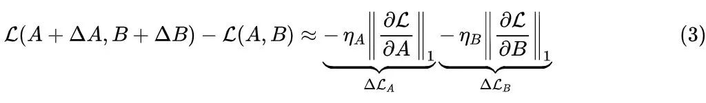
Where is the respective learning rate, the conclusion of “LoRA+” is that .Substituting the increment of SignSGD (2) back into equation (1), we get
Here, is the norm, that is, the sum of the absolute values of all components. “Equivalent contribution” means that we hope the right side’s is consistent in order of magnitude.
Quick Derivation
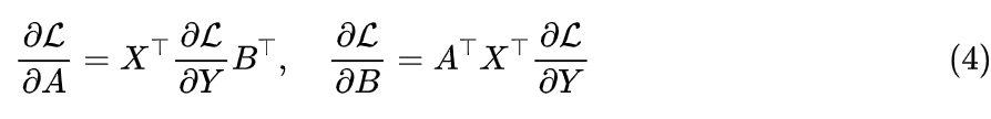
Further analysis requires determining the specific form of the gradient. Let Y=XAB, then we can derive:
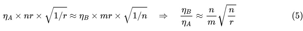
Readers unfamiliar with matrix differentiation may be confused by the derivation of the above result; in fact, I am not very familiar with it either, but there is a simple trick to use. For example, we know it is a matrix of shape (same shape as A), and similarly, it is a matrix of shape , and according to the chain rule of differentiation, it is not difficult to determine that it should be the product of , X, and B. Therefore, we think about how these three matrices can be multiplied to obtain a matrix of shape .After determining the specific form, we have a quick way to understand LoRA+. First, it is proportional to , which is the sum of the absolute values of nr components. If each component is roughly equivalent, this means is roughly proportional to nr; then, concerning B, it is once, which can be roughly regarded as the magnitude of each component being proportional to the magnitude of B’s components. Combining this gives that is simultaneously proportional to both nr and the magnitude of B; similarly, is also roughly proportional to both mr and the magnitude of A.Earlier, we mentioned in the “Numerical Stability” section that to ensure forward numerical stability, the magnitude of B should be greater than that of A (proportional to their approximate standard deviations), so to make and comparable in size, we should have approximately:
Considering that in practical use, m=n is often the case, we can simply denote it asHowever, it is not over yet; we need to check whether the results are self-consistent, as one of the conditions we used is “forward numerical stability”, which has so far only been an ideal assumption. How can we make the assumption as valid as possible? One way to overcome an assumption is to introduce another assumption:In the Adam optimizer, if the ratio of the learning rates of two parameters is , then after long-term training, the ratio of the magnitudes of these two parameters will also be .According to Adam’s approximation (2), the order of magnitude of each update increment is indeed proportional to the learning rate, but the total update result is not simply the sum of each step, so this assumption feels like “it seems somewhat reasonable, but not entirely so”. However, that’s okay; assumptions are usually like this; a bit of reason is enough, and the rest relies on faith.Under this assumption, if we train with a learning rate of , then the ratio of the magnitudes of parameters B and A will also be , and since we previously expected them to have approximately the same standard deviation , this ratio is exactly , leading to a completely self-consistent result!The results in the original paper differ slightly from the above, giving the answer as . This is because the original paper considers equal increments for Y, but Y is merely the output of the model layer and does not represent the final performance, thus being inappropriate.Although the original paper also attempts to relate the increment of Y to that of , it does not elaborate on the calculations, leading to deviations in the results. Additionally, the derivation in the original paper is, in principle, only applicable to the special case of b=1 and r=1, while the general case of b > 1 and r > 1 is directly inherited, meaning the analysis process is actually not sufficiently general.Of course, whether it is or is not particularly important; in practice, it still needs to be tuned. However, LoRA+ has conducted experiments on models of various sizes, with r generally set to 8, and n varying from 768 to 4096. The final recommended default learning rate ratio is , which is roughly similar to , thus the optimal value is closer to than to .
Article Summary
In this article, we introduced and derived a result called “LoRA+”, which supports the inherent asymmetry of the two low-rank matrices A and B in LoRA. Regardless of which matrix is initialized to all zeros, the learning rate of B should be set greater than that of A to achieve better performance.
How can we make more quality content reach the reader group with a shorter path, reducing the cost for readers to find quality content? The answer is: people you don’t know.
There are always some people you don’t know who know what you want to know. PaperWeekly may serve as a bridge, facilitating collisions of academic inspiration from scholars with different backgrounds and directions, sparking more possibilities.
PaperWeekly encourages university laboratories or individuals to share various quality content on our platform, which can include latest paper interpretations, analysis of academic hotspots, research insights, or competition experience explanations. Our only goal is to make knowledge flow genuinely.
📝 Basic Submission Requirements:
• The article must be an original work, not previously published in public channels. If it is an article published or to be published on other platforms, please clearly indicate
• Manuscripts are recommended to be written in markdown format, and images in the text should be sent as attachments, requiring clear images without copyright issues
• PaperWeekly respects the author’s right to attribution and will provide competitive remuneration for each accepted original first publication, based on a tiered system according to the article’s reading volume and quality