?p=8145

As the name suggests, time series data is a type of data that changes over time. For example, temperature over 24 hours, prices of various products over a month, or stock prices of a specific company over a year.(Click on “Read the original text” at the end for the complete code data).

Advanced deep learning models such as Long Short-Term Memory (LSTM) networks can capture patterns in time series data, making them suitable for predicting future trends in the data. In this article, you will see how to use the LSTM algorithm to make future predictions using time series data.

Related Video

Dataset and Problem Definition

Let’s first import the required libraries and then load the dataset:

import matplotlib.pyplot as plt
# Load the dataset into our program

data.head()

Output:

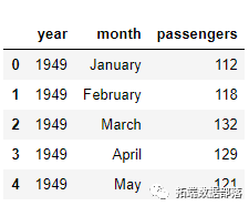
The dataset has three columns: year, month, and passengers. The passengers column contains the total number of travelers for the specified month. Let’s output the dimensions of the dataset:

data.shape

Output:

(144, 3)

You can see that the dataset has 144 rows and 3 columns, which means it contains 12 years of passenger travel records.

The task is to predict the number of travelers for the most recent 12 months based on the previous 132 months. Remember, we have records for 144 months, meaning the first 132 months of data will be used to train our LSTM model, and the model’s performance will be evaluated using the values from the most recent 12 months.

Let’s plot the monthly frequency of passengers. The following script plots the frequency of passengers per month:

plt.grid(True)
plt.autoscale(axis='x', tight=True)
plt.plot(data['passengers'])

Output:

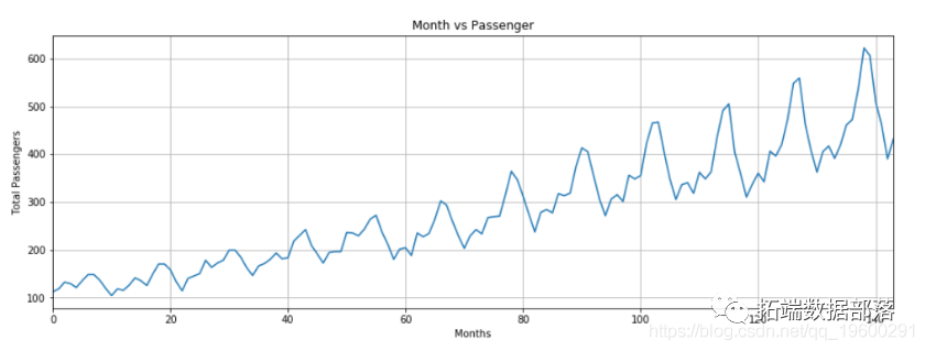
The output shows that the average number of passengers traveling by air has increased over the years. The number of passengers traveling within a year fluctuates, which makes sense as the number of travelers during summer or winter holidays is higher compared to other times of the year.

Click the title to check previous content

[Video] Python LSTM Long Short-Term Memory Neural Network for Unstable Rainfall Time Series Prediction Analysis | Data Sharing

Swipe left and right to see more

Data Preprocessing

The column types in the dataset are object, as shown in the following code:

data.columns

Output:

Index(['year', 'month', 'passengers'], dtype='object')

The first step is to change the type of the passengers column to float.

all_data = data['passengers'].values.astype(float)

Now, if we output the all_data numpy array, we should see the following floating-point values:

print(all_data)

The first 132 records will be used to train the model, and the last 12 records will serve as the test set. The following script splits the data into training and testing sets.

test_data_size = 12
train_data = all_data[:-test_data_size]
test_data = all_data[-test_data_size:]

Now let’s output the lengths of the test and training sets:

Output:

132
12

If we now output the test data, you will see it contains the last 12 records from the all_data numpy array:Output:

[417. 391.... 390. 432.]

Our dataset is currently not normalized. The total number of passengers in the initial years is much lower than in the later years. Normalizing data for time series prediction is very important. It is essential to scale the data between a minimum and maximum value within a certain range. We will use the MinMaxScaler class from the sklearn.preprocessing module to scale the data.

The following code normalizes the data with a maximum value of 1 and a minimum value of -1.

MinMaxScaler(feature_range=(-1, 1))

Output:

[[-0.96483516]
......
 [0.33186813]
 [0.13406593]
 [0.32307692]]

You can see that the dataset values are now between -1 and 1.

It is important to mention that data normalization is only applied to the training data and not to the test data. If normalization is applied to the test data, some information may leak from the training set to the test set.

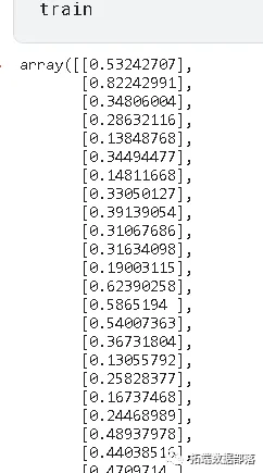
The final preprocessing step is to convert our training data into sequences and corresponding labels.

You can use any sequence length depending on domain knowledge. However, in our dataset, using a sequence length of 12 is convenient because we have monthly data, and there are 12 months in a year. If we had daily data, a better sequence length would be 365, which is the number of days in a year. Therefore, we will set the input sequence length for training to 12.

Next, we will define a function called create_inout_sequences. This function will take the raw input data and return a list of tuples. In each tuple, the first element will contain a list of 12 items corresponding to the number of passengers traveling within 12 months, and the second element of the tuple will contain one item, which is the number of passengers in the 12 + 1 month.

If you output the length of the train_inout_seq list, you will see it contains 120 items. This is because although the training set contains 132 elements, the sequence length is 12, meaning the first sequence consists of the first 12 items, and the 13th item is the label for the first sequence. Similarly, the second sequence starts from the second item and ends at the 13th item, with the 14th item being the label for the second sequence, and so on.

Now let’s output the first 5 items of the train_inout_seq list:

Output:

[(tensor([-0.9648, -0.9385, -0.8769, -0.8901, -0.9253, -0.8637, -0.8066, -0.8066,          -0.8593, -0.9341, -1.0000, -0.9385]), tensor([-0.9516])),
 (tensor([-0.9385, -0.8769, -0.8901, -0.9253, -0.8637, -0.8066, -0.8066, -0.8593,
          -0.9341, -1.0000, -0.9385, -0.9516]),
tensor([-0.9033])),
 (tensor([-0.8769, -0.8901, -0.9253, -0.8637, -0.8066, -0.8066, -0.8593, -0.9341,
          -1.0000, -0.9385, -0.9516, -0.9033]), tensor([-0.8374])),
 (tensor([-0.8901, -0.9253, -0.8637, -0.8066, -0.8066, -0.8593, -0.9341, -1.0000,
          -0.9385, -0.9516, -0.9033, -0.8374]), tensor([-0.8637])),
 (tensor([-0.9253, -0.8637, -0.8066, -0.8066, -0.8593, -0.9341, -1.0000, -0.9385,
          -0.9516, -0.9033, -0.8374, -0.8637]), tensor([-0.9077]))]

You will see that each item is a tuple where the first element consists of 12 items of the sequence, and the second element of the tuple contains the corresponding label.

Creating the LSTM Model

We have preprocessed the data, and now it’s time to train our model. We will define a class LSTM that inherits from the nn.Module class of the PyTorch library.

Let me summarize the above code. The constructor of the LSTM class takes three parameters:

input_size: corresponds to the number of features in the input. Although our sequence length is 12, we only have 1 value per month, which is the total number of passengers, so the input size is 1.
hidden_layer_size: specifies the number of hidden layers and the number of neurons in each layer. We will have one layer with 100 neurons.
output_size: the number of items in the output. Since we want to predict the number of passengers for the next month, the output size is 1.

Next, in the constructor, we create variables hidden_layer_size, lstm, linear, and hidden_cell. The LSTM algorithm takes three inputs: the previous hidden state, the previous cell state, and the current input. The hidden_cell variable contains the previous hidden state and cell state. The lstm and linear layer variables are used to create the LSTM and linear layers.

Inside the forward method, the input_seq is passed as a parameter, which is first passed to the lstm layer. The output of the lstm layer is the hidden state and cell state for the current time step, as well as the output. The output of the lstm layer will be passed to the linear layer. The expected number of passengers is stored in the last item of the predictions list and returned to the calling function. The next step is to create an object of the LSTM() class, define the loss function and optimizer. Since we are solving a regression problem,

class LSTM(nn.Module):
    def __init__(self, input_size=1, hidden_layer_size=100, output_size=1):
        super().__init__()
        self.hidden_layer_size = hidden_layer_size

Let’s output the model:

Output:

LSTM(
  (lstm): LSTM(1, 100)
  (linear): Linear(in_features=100, out_features=1, bias=True)
)

Training the Model

We will train the model for 150 epochs.

epochs = 150
for i in range(epochs):
    for seq, labels in train_inout_seq:
        optimizer.zero_grad()

Output:

epoch:   1 loss: 0.00517058
epoch:  26 loss: 0.00390285
epoch:  51 loss: 0.00473305
epoch:  76 loss: 0.00187001
epoch: 101 loss: 0.00000075
epoch: 126 loss: 0.00608046
epoch: 149 loss: 0.0004329932

Since weights are randomly initialized in PyTorch neural networks by default, you may get different values.

Making Predictions

Now that our model is trained, we can start making predictions.

You can compare the above values with the last 12 values of the train_data_normalized data list.

The test_inputs item will contain 12 items. In the for loop, these 12 items will be used to predict the first item in the test set, which is number 133. The predicted value will then be appended to the test_inputs list. In the second iteration, the last 12 items will again be used as input, and a new prediction will be made, and then the test_inputs will be appended again. Since there are 12 elements in the test set, this loop will run 12 times. At the end of the loop, the test_inputs list will contain 24 items. The last 12 items will be the predicted values for the test set. The following script is used to make predictions:

model.eval()
for i in range(fut_pred):
    seq = torch.FloatTensor(test_inputs[-train_window:])

If you output the length of the test_inputs list, you will see it contains 24 items. You can output the last 12 predicted items as follows:

It needs to be mentioned again that depending on the weights used to train the LSTM, you may get different values.

Since we normalized the training dataset, the predicted values are also normalized. We need to convert the normalized predicted values back to actual predicted values.

print(actual_predictions)

Now let’s plot the predicted values against the actual values. See the code below:

print(x)

In the above script, we create a list containing the values for the last 12 months. The index value for the first month is 0, so the index value for the last month is 143.

In the following script, we will plot the total number of passengers for 144 months along with the expected number of passengers for the last 12 months.

plt.autoscale(axis='x', tight=True)
plt.plot(flight_data['passengers'])
plt.plot(x, actual_predictions)
plt.show()

Output:

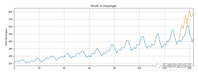
The predictions made by our LSTM are represented by the orange line. You can see that our algorithm is not very accurate, but it is still able to capture the upward trend and fluctuations in the total number of passengers traveling over the last 12 months. You can try using more epochs and more neurons in the LSTM layer to see if you can achieve better performance.

To better visualize the output, we can plot the actual and predicted number of passengers for the last 12 months as follows:

plt.plot(flight_data['passengers'][-train_window:])
plt.plot(x, actual_predictions)
plt.show()

Output:

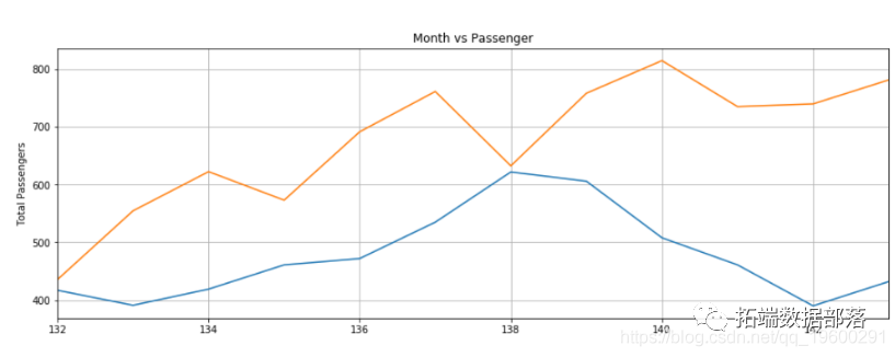
The predictions are not very accurate, but the algorithm is able to capture the trend that the number of passengers in the coming months should be higher than in previous months, with occasional fluctuations.

Conclusion

LSTM is one of the most widely used algorithms for solving sequence problems. In this article, we saw how to use LSTM for future predictions using time series data.

Click at the end“Read the original text”

to obtain the complete code data materials..

This article is excerpted from “Time Series Prediction Using LSTM and PyTorch in Python”.

Click the title to check previous content

PYTHON LSTM Neural Network for Time Series Prediction of Natural Gas Prices ExamplePython LSTM and XGBoost Sales Time Series Modeling Prediction Analysis on Store DataMatlab Deep Learning LSTM Neural Network for Text Data ClassificationRNN Recurrent Neural Network, LSTM Long Short-Term Memory Network for Long-Term Interest Rate PredictionCombining COVID-19 Pandemic Stock Price Prediction: ARIMA, KNN, and Neural Network Time Series AnalysisDeep Learning: Keras Simple Text Classification Analysis on News Group Data Using Neural NetworksUsing PyTorch Machine Learning Neural Network Classification to Predict Bank Customer Churn ModelPYTHON LSTM Neural Network Parameter Optimization Method for Time Series Shampoo Sales Data PredictionPython Keras Neural Network Sequential Model Regression Fitting Prediction, Accuracy Check, and Result VisualizationPython LSTM Neural Network for Unstable Rainfall Time Series Prediction AnalysisNeural Network Time Series Prediction in R: Multilayer Perceptron (MLP) and Extreme Learning Machine (ELM) Data Analysis ReportDeep Learning in R: Predicting Time Series Data with Keras Neural Network Regression ModelMatlab Deep Learning LSTM Neural Network for Text Data ClassificationR KERAS Deep Learning CNN Convolutional Neural Network Classification Recognition of Handwritten Digit Image Data (MNIST)Predicting Human Body Fat Percentage Data Using BP Neural Network in MATLABPredicting Bank Customer Churn Model Using PyTorch Machine Learning Neural Network Classification in PythonR Implementation of CNN (Convolutional Neural Network) Model for Regression Data AnalysisSAS Training Artificial Neural Network (ANN) Model Using Iris Dataset[Video] R Implementation of CNN (Convolutional Neural Network) Model for Regression Data AnalysisSimple Text Classification Using Neural Networks in PythonR Neural Network Improving Nelson-Siegel Model Fitting Yield Curve AnalysisR Recursive Neural Network RNN Temperature Time Series PredictionR Neural Network Model Predicting Vehicle Count Time SeriesR Neural Network Model Analyzing Student GradesClassifying Sequence Data Using Long Short-Term Memory (LSTM) Neural Network in MATLABR Implementation of Fitting Neural Network Prediction and Result VisualizationImplementing Neural Network Prediction of Stocks Using RUsing KERAS LSTM Recurrent Neural Network for Time Series Prediction in PYTHONPython Seq2Seq Model Example for NLP: Implementing Neural Network Machine Translation with KerasPython for NLP: Multi-label Text LSTM Neural Network Classification Using Keras

Time Series Prediction Using LSTM and PyTorch in Python

Full text link: http://tecdat.cn/?p=8145

Dataset and Problem Definition

Data Preprocessing

Creating the LSTM Model

Training the Model

Making Predictions

Conclusion

Related posts

Leave a Comment Cancel reply