Python | Typhoon GPI | Potential Intensity

Typhoon “Capricorn”

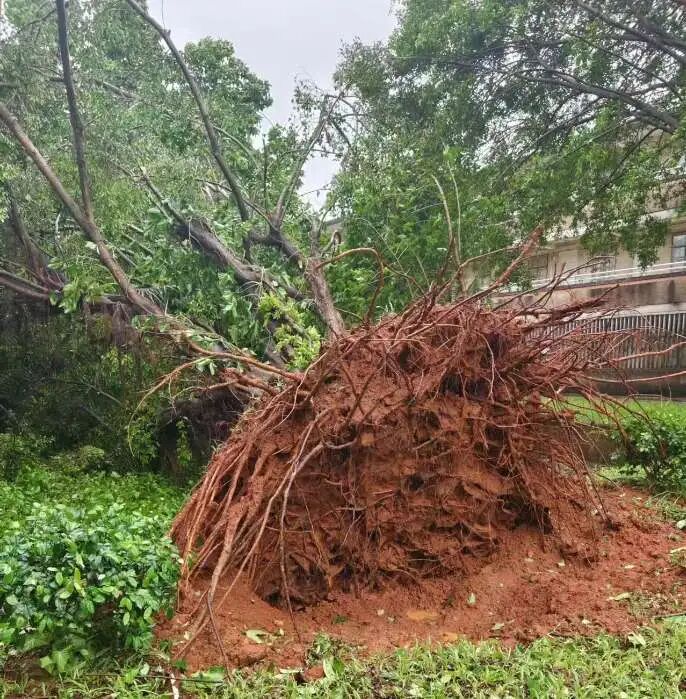
The “Capricorn” typhoon passed…

GPI

I often see or hear about GPI in some articles and group meetings, but I never knew what it was, so I spent half an hour to understand it.

Genesis Potential Index (GPI) is an index used to predict the likelihood of tropical cyclone (typhoon) formation.

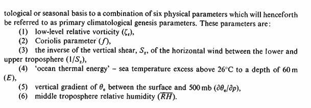
In 1979, Gray proposed six large-scale parameter factors closely related to TC formation and development.

Three Dynamic Factors

Corriolis parameter
Lower-level relative vorticity
Vertical wind shear

Three Thermodynamic Factors

Mid-level humidity
Mid-low level static stability
SST

Based on this, Emanuel and Nolan (2004) first proposed the GPI index:

Subsequently, Murakami et al. (2011) improved it by adding the 500 hPa vertical velocity:

In the formula,

is the absolute vorticity at 850 hPa, with units of ,
RH represents the relative humidity at 600 hPa, with units of %,
is the maximum potential intensity, representing the maximum wind speed that TC can reach under certain sea-atmosphere thermodynamic conditions, with units of (Emanuel, 1995; Emanuel et al., 2004),
is the vertical wind shear from 200 to 850 hPa, with units of ,
is the vertical velocity at 500 hPa, with units of Pa .

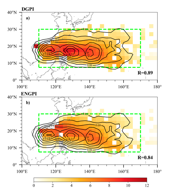
Another form of the GPI equation was proposed by the internationally renowned meteorologistWang Bin with the DGPI:

ENGPI mainly considers the environmentalthermodynamic factors, while DGPI emphasizes the role of large-scaledynamic factors.

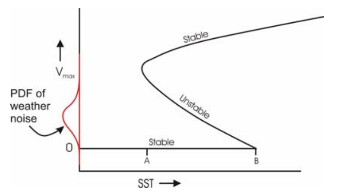
Potential Intensity

Except for DGPI, the above three formulas all have aMaximum Potential Intensity (Potential Intensity, PI), which is generally calculated using the BE02 algorithm. This algorithm was originally written in FORTRAN by Professor Kerry Emanuel (MIT) and later in MATLAB. Kerry’s original MATLAB code (pcmin.m) is located at:<span>http://texmex.mit.edu/pub/emanuel/TCMAX</span>.

The formula for the PI BE02 algorithm is:

Where,

is the absolute sea surface temperature.
is the average outflow temperature.
is the enthalpy exchange coefficient.
is the drag coefficient.
is the convective available potential energy when saturated moist air rises from sea level.
is the effective convective potential energy when boundary layer air rises.

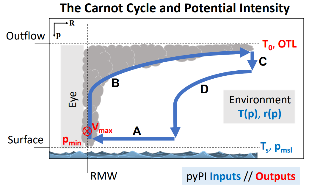
pyPI

Python can use the tcpypi library to calculate the maximum potential intensity. Installation:

pip install tcpypi

Usage example:

import sys
sys.path.append(sys.path[0]+'/..')
import numpy as np
import xarray as xr
import matplotlib
import matplotlib.pyplot as plt
import time
# load PI calculation module
from tcpyPI import pi

# change default figure font settings
font = {'family' : 'sans-serif',
        'weight' : 1,
        'size'   : 16}

matplotlib.rc('font', **font)

# data location
dat_loc='../data/sample_data.nc'
# load and view netcdf file
ds = xr.open_dataset(dat_loc)

# store the data in numpy arrays
SST,MSL,Ta,R,P=np.asarray(ds.sst),np.asarray(ds.msl),np.asarray(ds.t),np.asarray(ds.q),np.asarray(ds.p)

# find the sizes of the the arrays
nlat,nlon=ds.sst.sizes['lat'],ds.sst.sizes['lon']
# create arrays to store data
VMAXp,PMINp,TOp,LNBp=np.zeros((12,nlat,nlon),dtype='float64'),np.zeros((12,nlat,nlon),dtype='float64'), 
    np.zeros((12,nlat,nlon),dtype='float64'),np.zeros((12,nlat,nlon),dtype='float64')
IFLp=np.zeros((12,nlat,nlon),dtype='float64')
# fill with missing data
VMAXp[:],PMINp[:],TOp[:],LNBp[:],IFLp[:]=np.nan,np.nan,np.nan,np.nan,np.nan
# (VMAX,PMIN,IFL,TO,LNB)=pi(sst1,msl1,p1,t1,q1,CKCD=0.9,ascent_flag=0,diss_flag=1,V_reduc=0.8,ptop=50,miss_handle=1)

# time the loop
start = time.time()

# loop over the data grid and calculate PI
for m in range(12):
    for x in range(nlon):
        for y in range(nlat):
            if (SST[m,y,x]>0.0):
                (VMAXp[m,y,x],PMINp[m,y,x],IFLp[m,y,x],TOp[m,y,x],LNBp[m,y,x]) = pi( 
                    SST[m,y,x],MSL[m,y,x],P,Ta[m,:,y,x],R[m,:,y,x],
                    CKCD=0.9,ascent_flag=0,diss_flag=1,V_reduc=0.8,ptop=50,miss_handle=1)

end = time.time()
print(end - start)

# calculate the difference between Python and MATLAB
diff_VMAX=VMAXp-ds.Vmax

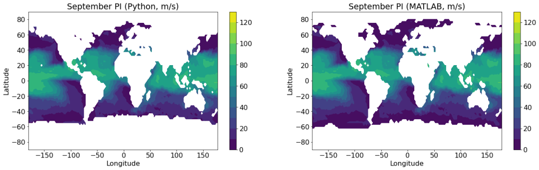
# plot both side by side in September
clevels=np.arange(0,140,10)
plt.figure(figsize=(22,6))
plt.subplot(1,2,1)
plt.contourf(ds.lon,ds.lat,VMAXp[8,:,:],clevels)
plt.xlabel(ds.lon.standard_name)
plt.ylabel(ds.lat.standard_name)
plt.title('September PI (Python, m/s)')
plt.colorbar()

plt.subplot(1,2,2)
plt.contourf(ds.lon,ds.lat,ds.Vmax.isel(month=8),clevels)
plt.xlabel(ds.lon.standard_name)
plt.ylabel(ds.lat.standard_name)
plt.title('September PI (MATLAB, m/s)')
plt.colorbar()
plt.show()

plt.figure(figsize=(10,6))
clevels=np.linspace(-0.02,-0.0,11)
plt.contourf(ds.lon,ds.lat,diff_VMAX.isel(month=8),levels=clevels)
plt.xlabel(ds.lon.standard_name)
plt.ylabel(ds.lat.standard_name)
plt.title('September PI Difference (Python$-$MATLAB, m/s)')
plt.colorbar()
plt.show()

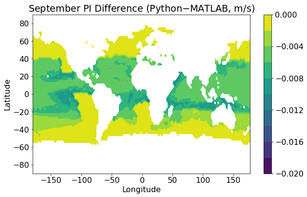
The results are quite close.

References

Gray, W. M. 1979: Hurricanes: Their formation, structure and likely role in the general circulation. Meteorology over the Tropical Oceans, D. B. Shaw, Ed., Royal Meteorological Society, 155–218.
Emanuel K A, Nolan D S. 2004. Tropical cyclone activity and global climate [J]. Bull. Amer. Meteor. Soc., 85(5): 666−667.
Murakami, H., Wang, B., Kitoh, A., 2011. Future Change of Western North Pacific Typhoons: Projections by a 20-km-Mesh Global Atmospheric Model*. J. Clim. 24, 1154–1169. https://doi.org/10.1175/2010JCLI3723.1
Wang, B., & Murakami, H. (2020). Dynamic genesis potential index for diagnosing present-day and future global tropical cyclone genesis. Environmental Research Letters, 15(11), 114008. https://doi.org/10.1088/1748-9326/abbb01
Gilford, D. M.: pyPI (v1.3): Tropical Cyclone Potential Intensity Calculations in Python, Geosci. Model Dev., 14, 2351–2369, https://doi.org/10.5194/gmd-14-2351-2021, 2021.
Bister, M., Emanuel, K.A., 2002. Low frequency variability of tropical cyclone potential intensity 1. Interannual to interdecadal variability. J. Geophys. Res. Atmospheres 107. https://doi.org/10.1029/2001JD000776
Wang, C.,Wang, Y., Wang, B., Wu, L., Zhao, H., Cao, J. (2023). Opposite skills of ENGPI and DGPI in depicting decadal variability of tropical cyclone genesis over the western North Pacific. Journal of climate, 36(24): 8713–8721. doi:https://doi.org/10.1175/JCLI-D-23-0201.1.

Previous Issues

Python | MJO | Phase Diagram
Python | Longitude Conversion Between Hemispheres
Python | Atmospheric Science | Partial Correlation
37 CMIP6 Models Convection Parameterization Schemes
Python | Solving cmaps Library Error Issues
Python | Batch Download of NCEP2 Reanalysis Data
Python | North Atlantic Oscillation | NAO Index | EOF