Essential Python Libraries for Operations Research Optimization: A Comprehensive Analysis

In the era of artificial intelligence and Industry 4.0, operations research technology has become the core engine for enhancing decision-making efficiency. Python, with its powerful scientific computing ecosystem, has nurtured numerous specialized optimization libraries. This article introduces 8 major Python operations research tools, covering linear programming, integer programming, combinatorial optimization, and other comprehensive needs to help you build efficient decision-making systems.

1. SciPy: The Swiss Army Knife of Basic Optimization

Key Features

• Provides the <span>scipy.optimize</span> module, supporting linear programming (LP) and nonlinear programming (NLP)
• Core functions: <span>linprog()</span> (linear programming), <span>minimize()</span> (nonlinear optimization)
• Advantages: Zero configuration usage, perfectly integrates into scientific computing workflows

import numpy as np
from scipy.optimize import linprog

# Define the problem: maximize 3x + 5y, subject to x + 2y ≤ 100, x,y ≥ 0 and integers
def solve_integer_problem():
    # 1. Solve continuous linear programming (as a reference for integer solutions)
    res = linprog(
        c=[-3, -5],  # Coefficients of the objective function (negated for maximization)
        A_ub=[[1, 2]],  # Constraint coefficient matrix
        b_ub=[100],     # Upper limit of constraints
        bounds=[(0, None), (0, None)],  # Non-negative constraints for variables
        method='highs'
    )
    
    if not res.success:
        return "Failed to solve: No feasible solution found"
    
    # 2. Generate candidate integer solutions near the continuous solution
    x_cont, y_cont = res.x
    candidates = [(x, y) for x in range(max(0, int(x_cont)-2), int(x_cont)+3)
                        for y in range(max(0, int(y_cont)-2), int(y_cont)+3)
                        if x + 2*y <= 100]  # Filter solutions that satisfy the constraints
    
    # 3. Select the optimal integer solution
    best_x, best_y = max(candidates, key=lambda xy: 3*xy[0] + 5*xy[1])
    max_val = 3*best_x + 5*best_y
    
    return f"Optimal integer solution:\nx = {best_x}, y = {best_y}\nMaximum value of the objective function = {max_val}"

# Execute and print the result
print(solve_integer_problem())

Applicable Scenarios: Algorithm prototype verification, teaching cases, small engineering problems.

2. Gurobi: Industrial-Grade High-Performance Engine

Core Advantages

• Peak commercial solver: Mixed Integer Programming (MIP) solving speed is leading
• Supports distributed computing, optimizing millions of variables
• Free licenses for academic users

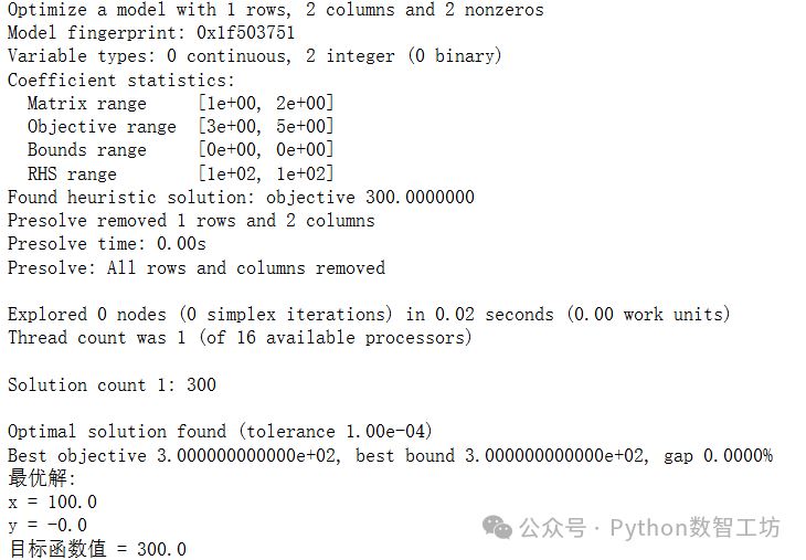
from gurobipy import Model, GRB

# Create model
model = Model("SupplyChain")

# Add integer variables
x = model.addVar(vtype=GRB.INTEGER, name="x")
y = model.addVar(vtype=GRB.INTEGER, name="y")
# Add constraints
model.addConstr(x + 2*y <= 100, "ResourceConstraint")

# Set objective function (maximize)
model.setObjective(3*x + 5*y, GRB.MAXIMIZE)


# Execute optimization
model.optimize()

# Check if optimization was successful
if model.status == GRB.OPTIMAL:
    # Output optimal variable values
    print(f"Optimal solution:")
    print(f"x = {x.x}")
    print(f"y = {y.x}")
    print(f"Objective function value = {model.objVal}")
else:
    print("No optimal solution found")

Typical Applications: Supply chain network design, financial portfolio optimization

3. PuLP: Lightweight Modeling Tool

Notable Features

• Syntax close to mathematical expressions: <span>prob += 3*x1 + 4*x2</span>
• Seamless integration withCBC, GLPK and other open-source solvers
• Models can be exported in LP/MPS standard format

import pulp

# Create problem instance, specified as a maximization problem
model = pulp.LpProblem("SupplyChain", pulp.LpMaximize)

# Define decision variables (non-negative integers)
x = pulp.LpVariable('x', lowBound=0, cat='Integer')  # lowBound=0 indicates x≥0
y = pulp.LpVariable('y', lowBound=0, cat='Integer')  # cat='Integer' specifies as integer variable

# Set objective function
model += 3 * x + 5 * y, "TotalProfit"  # The second parameter is the name of the objective function

# Add constraints
model += x + 2 * y <= 100, "ResourceConstraint"  # Constraint name is "ResourceConstraint"

# Solve the model
status = model.solve(pulp.PULP_CBC_CMD(msg=0))  # msg=0 indicates no solver log displayed

# Output solving status
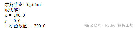
print(f"Solving status: {pulp.LpStatus[status]}")

# Output optimal solution
if pulp.LpStatus[status] == "Optimal":
    print(f"Optimal solution:")
    print(f"x = {x.varValue}")
    print(f"y = {y.varValue}")
    print(f"Objective function value = {pulp.value(model.objective)}")
else:
    print("No optimal solution found")

Best Scenarios: Teaching demonstrations, small production scheduling optimization

4. Pyomo: Enterprise-Level Modeling Framework

Architectural Advantages

• Separation of models and solvers: Supports Gurobi/CPLEX/GLPK
• Provides abstract models (AbstractModel) and concrete models (ConcreteModel)
• Strong capability to express complex constraint systems

from pyomo.environ import ConcreteModel, Var, Objective, Constraint, Integers, maximize, SolverFactory

# Create a concrete model instance
model = ConcreteModel(name="SupplyChain")

# Define decision variables (non-negative integers)
model.x = Var(domain=Integers, bounds=(0, None), name="x")  # bounds=(0, None) indicates x≥0
model.y = Var(domain=Integers, bounds=(0, None), name="y")  # domain=Integers specifies as integer variable

# Define objective function (maximize)
def objective_rule(model):
    return 3 * model.x + 5 * model.y
model.objective = Objective(rule=objective_rule, sense=maximize, name="TotalProfit")

# Define constraints
def constraint_rule(model):
    return model.x + 2 * model.y <= 100
model.constraint = Constraint(rule=constraint_rule, name="ResourceConstraint")

# Note/Attention, select solver and solve (using CBC solver, needs to be installed in advance)
solver = SolverFactory('cbc')  # Using open-source CBC solver
results = solver.solve(model)

# Output solving status
print(f"Solving status: {results.solver.status}")
print(f"Termination condition: {results.solver.termination_condition}")

# Output optimal solution
if results.solver.termination_condition == 'optimal':
    print("\nOptimal solution:")
    print(f"x = {model.x.value}")
    print(f"y = {model.y.value}")
    print(f"Objective function value = {model.objective.value}")
else:
    print("No optimal solution found")

Industrial Applications: Chemical process optimization, power system scheduling

5. OR-Tools: Google’s Open Source Combinatorial Optimization Tool

Breakthrough Capabilities

• Specializes in NP-Hard problems: Vehicle Routing Problem (VRP), scheduling problems
• Built-in heuristic algorithms: Large Neighborhood Search (LNS)

from ortools.linear_solver import pywraplp

# Create solver (using GLOP linear programming solver, built into OR-Tools)
solver = pywraplp.Solver.CreateSolver("SCIP")  # SCIP is the solver for integer programming in OR-Tools

# Define integer variables (non-negative)
x = solver.IntVar(0, solver.infinity(), "x")  # IntVar indicates integer variable, first parameter is lower bound
y = solver.IntVar(0, solver.infinity(), "y")

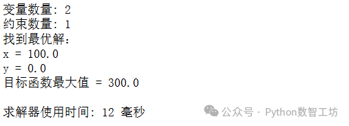
print(f"Number of variables: {solver.NumVariables()}")

# Add constraints x + 2y ≤ 100
constraint = solver.Constraint(-solver.infinity(), 100)  # Constraint range (-∞, 100]
constraint.SetCoefficient(x, 1)  # Coefficient of x is 1
constraint.SetCoefficient(y, 2)  # Coefficient of y is 2

print(f"Number of constraints: {solver.NumConstraints()}")

# Define objective function: maximize 3x + 5y
objective = solver.Objective()
objective.SetCoefficient(x, 3)
objective.SetCoefficient(y, 5)
objective.SetMaximization()  # Set as maximization problem

# Solve the problem
status = solver.Solve()

# Output results
if status == pywraplp.Solver.OPTIMAL:
    print("Found optimal solution:")
    print(f"x = {x.solution_value()}")
    print(f"y = {y.solution_value()}")
    print(f"Maximum value of the objective function = {objective.Value()}")
else:
    print("No optimal solution found")

# Output solver information
print(f"\nSolver time: {solver.WallTime()} milliseconds")

6. GEKKO: Expert in Dynamic System Optimization

Unique Value

• Supports differential algebraic equations (DAE) optimization
• Built-in solvers like APOPT, IPOPT for nonlinear optimization
• Powerful tool for control system design

from gekko import GEKKO

# Create model
m = GEKKO(remote=False)  # remote=False indicates using local solver

# Define integer variables (non-negative)
x = m.Var(integer=True, lb=0, name='x')  # integer=True specifies as integer variable, lb=0 sets lower bound to 0
y = m.Var(integer=True, lb=0, name='y')

# Set objective function (maximize 3x + 5y)
# Gekko defaults to minimization, so we achieve maximization by negating
m.Maximize(3*x + 5*y)

# Add constraints
m.Equation(x + 2*y <= 100)

# Solve model
m.solve(disp=False)  # disp=False does not display detailed solving process

# Output results
print("Optimal solution:")
print(f"x = {x.value[0]}")
print(f"y = {y.value[0]}")
print(f"Maximum value of the objective function = {m.options.OBJFCNVAL * -1}")  # Multiply by -1 to restore maximum value

Engineering Applications: Chemical process control, robot trajectory optimization

7. Scikit-opt: A Treasure Trove of Metaheuristic Algorithms

Core Features

• Integrates 7 types of heuristic algorithms: Genetic algorithms, simulated annealing, etc.
• Supports GPU acceleration for efficient solving of large-scale optimization problems

from sko.GA import GA
import numpy as np
import matplotlib.pyplot as plt
# Objective function: maximize 3x + 5y (converted to minimization problem, returning negative value)
def objective_func(x):
    return -(3 * x[0] + 5 * x[1])

# Constraints: x + 2y ≤ 100 (returns value ≥ 0 when constraints are satisfied)
def constraint_func(x):
    return 100 - (x[0] + 2 * x[1])

# Create genetic algorithm instance
ga = GA(
    func=objective_func,          # Objective function
    n_dim=2,                      # Variable dimensions (x and y)
    size_pop=500,                 # Population size
    max_iter=2000,                # Number of iterations
    lb=[0, 0],                    # Variable lower bounds (x≥0, y≥0)
    ub=[100, 50],                 # Variable upper bounds (estimated based on constraints)
    prob_mut=0.005,               # Mutation coefficient, default 0.001
    constraint_eq=[constraint_func],  # Constraints
)

# Execute optimization
best_x, best_y = ga.run()

# Output results
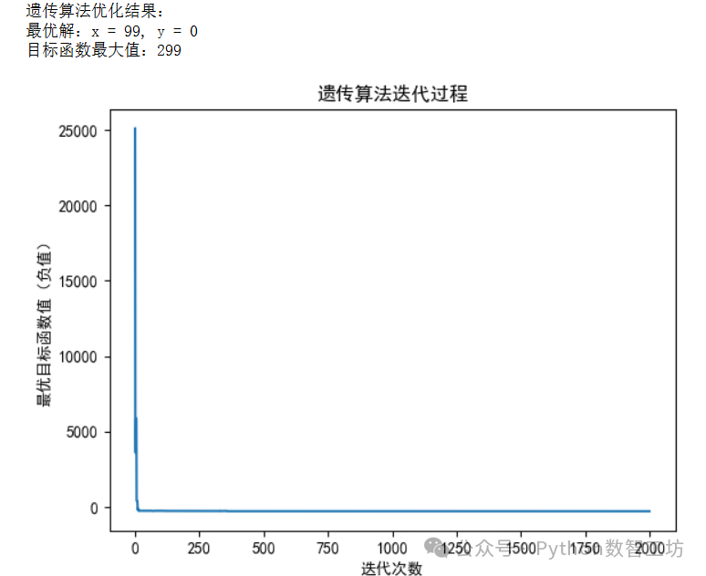
print("Genetic algorithm optimization results:")
print(f"Optimal solution: x = {int(best_x[0])}, y = {int(best_x[1])}")
print(f"Maximum value of the objective function: {int(-best_y)}")  # Restore to positive value

# Plot iteration curve

plt.rcParams['font.sans-serif'] = ['SimHei']  # Set Chinese font
plt.plot(ga.generation_best_Y)
plt.title("Genetic Algorithm Iteration Process")
plt.xlabel("Number of Iterations")
plt.ylabel("Optimal Objective Function Value (Negative)")
plt.show()

Innovative Scenarios: Hyperparameter optimization for neural networks, global optimization of non-convex functions

8. CVXPY: A Pythonic Solution for Convex Optimization

Technical Highlights

• Complies with Disciplined Convex Programming (DCP) rules
• Automatically derives standard forms for convex optimization problems

import cvxpy as cp
from cvxpy.error import SolverError  # Import specific exception class

# Define integer variables (correctly specify variable types)
x = cp.Variable(integer=True, name="x")
y = cp.Variable(integer=True, name="y")

# Define objective function: maximize 3x + 5y
objective = cp.Maximize(3 * x + 5 * y)

# Define constraints:
constraints = [
    x + 2 * y <= 100,  # Resource constraint
    x >= 0,             # Non-negative constraint
    y >= 0              # Non-negative constraint
]

# Create optimization problem
problem = cp.Problem(objective, constraints)

# Define order of solver attempts
solvers = [
    ("CBC", cp.CBC),
    ("GLPK_MI", cp.GLPK_MI),
    ("ECOS_BB", cp.ECOS_BB),
    ("SCIP", cp.SCIP)
]

result = None
solver_used = None

# Attempt multiple solvers
for solver_name, solver in solvers:
    try:
        result = problem.solve(solver=solver, verbose=False)
        solver_used = solver_name
        # Check if optimal solution was obtained
        if problem.status == cp.OPTIMAL:
            break
    except SolverError:
        print(f"Solver {solver_name} unavailable, trying next...")
    except Exception as e:
        print(f"Solver {solver_name} error: {str(e)}")

# Output solving results
print(f"\nSolver used: {solver_used or 'No available solver'}")
print(f"Solving status: {problem.status}")

if problem.status == cp.OPTIMAL:
    # Ensure integer values are obtained (round directly)
    x_val = int(round(x.value))
    y_val = int(round(y.value))
    
    print("\nOptimal solution:")
    print(f"x = {x_val}")
    print(f"y = {y_val}")
    print(f"Maximum value of the objective function = {round(objective.value)}")  # Use objective.value for more accuracy
elif problem.status == cp.INFEASIBLE:
    print("Problem infeasible, no solution")
elif problem.status == cp.UNBOUNDED:
    print("Problem unbounded, solution is infinite")
else:
    print("No optimal solution found, please check solver installation and problem settings")
    print(f"Last attempted results: x={x.value}, y={y.value}")

Advantage Areas: Portfolio optimization, signal processing

Tool Selection Matrix

Library Name	Optimization Type	Typical Problem Scale	Learning Curve
SciPy	LP/NLP	<10³ variables	Gentle
Gurobi	MIP/QP/NLP	>10⁶ variables	Moderate
PuLP	LP/IP	<10⁴ variables	Gentle
Pyomo	LP/MIP/NLP	10³-10⁶ variables	Steep
OR-Tools	Combinatorial Optimization	Path/Scheduling Problems	Moderate
GEKKO	Dynamic Optimization	DAE Systems	Professional
Scikit-opt	Heuristic Optimization	Complex Non-Convex Problems	Moderate
CVXPY	Convex Optimization	<10⁴ variables	Moderate

❝

Selection Notes:

• Mathematical programming problems: Preferred Gurobi/Pyomo
• Path scheduling optimization: OR-Tools
• Dynamic control systems: GEKKO
• Algorithm research verification: Scikit-opt/SciPy

Future Trends

With the integration of quantum computing and AI, a new generation of optimization libraries such as Qiskit Optimization (quantum optimization) and Optuna (hyperparameter optimization) are emerging. It is recommended to pay attention to the following directions:

1. Cloud-native optimization platforms: Integrated solving services from AWS/GCP
2. AutoML + optimization integration: Intelligent automatic parameter tuning
3. GPU parallel optimization: Thousands of times acceleration for large-scale problem solving