Multi-Layer Perceptron (MLP) Overview

MLP, short for Multi-Layer Perceptron, also known as Feedforward Neural Network. It is one of the most fundamental and core models in deep learning, which can be understood as a network composed of multiple layers of “neurons”.

1. Core Idea of MLP: Overcoming the Limitations of Single-Layer Perceptron

To understand MLP, one must first understand its predecessor – Perceptron.

Single-Layer Perceptron:

Structure: Only an input layer and an output layer.
Function: Essentially a linear classifier. It performs binary classification on data using a linear function (e.g., w*x + b) and an activation function (e.g., step function).
Critical Limitation: It cannot solve linearly inseparable problems, the most classic example being the “XOR” problem. No matter how a straight line is drawn, it cannot perfectly separate the two classes of points in the XOR problem.

MLP’s Breakthrough:

MLP introduces one or more hidden layers between the input layer and the output layer.
Each hidden layer consists of multiple neurons and is equipped with non-linear activation functions.
This “deep” structure allows MLP to approximate any complex continuous function by combining multiple simple linear and non-linear transformations, thus solving non-linear problems.

2. Basic Structure of MLP

A standard MLP typically consists of three parts:

Input Layer:

Responsible for receiving raw data. The number of neurons in this layer usually equals the number of input features.
This layer has no computational function, only responsible for data distribution.

Hidden Layers:

Linear Computation: z = w * x + b, where w is the weight, x is the input (from the output of the previous layer or input layer), and b is the bias.
Non-Linear Transformation: a = f(z), where f is the activation function. This step is crucial as it introduces non-linearity, enabling the network to learn complex patterns.

This is the core of MLP. There can be one or more layers.
Each hidden layer contains several neurons.
Each neuron does two things:

Output Layer:

Binary Classification: 1 neuron (using Sigmoid activation function).
Multi-Class Classification: N neurons (equal to the number of classes, using Softmax activation function).
Regression: 1 or more neurons (usually without activation function, or using linear activation function).

Produces the final prediction result.
The number of neurons depends on the task type:

3. Detailed Explanation of Key Components

1. Activation Function

This is the core of MLP’s ability to learn non-linear relationships. Without it, even the deepest networks are equivalent to a linear model. Common activation functions include:

Sigmoid: f(z) = 1 / (1 + e^{-z}), compresses output to (0, 1). Commonly used in the past, now mostly used in the output layer for binary classification.
Tanh: f(z) = (e^z - e^{-z}) / (e^z + e^{-z}), compresses output to (-1, 1). Its output is zero-centered and usually performs slightly better than Sigmoid.
ReLU (Rectified Linear Unit): f(z) = max(0, z). This is currently the most commonly used activation function because it effectively mitigates the vanishing gradient problem and is very fast to compute.
Softmax: Commonly used in multi-class output layers, it compresses the outputs of all neurons into a probability distribution, with the sum of all output values equal to 1.

2. Forward Propagation

The process where data starts from the input layer, passes through hidden layers, and finally reaches the output layer to produce results. Calculation process:output = activation function(weight * input + bias)

3. Loss Function

Used to measure the difference between the model’s predicted value ŷ and the true value y. Common loss functions include:

Mean Squared Error (MSE): Commonly used for regression problems.
Cross-Entropy Loss: Commonly used for classification problems.

4. Backpropagation and Optimizer

This is the learning mechanism of MLP.

Backpropagation: Using the chain rule, the loss is propagated backward from the output layer to the input layer to compute the gradient of the loss function with respect to each weight (w) and bias (b), indicating the direction and magnitude of parameter adjustments.
Optimizer: Uses the computed gradients to update the weights and biases in the network to minimize the loss function. The most commonly used optimizer is Gradient Descent and its variants (like Adam, SGD with Momentum, etc.). The update formula can be simplified to:w_new = w_old - learning_rate * gradient

The training process involves repeatedly performing the cycle of “forward propagation -> compute loss -> backpropagation -> update parameters”.

4. Advantages and Disadvantages of MLP

Advantages:

Powerful Function Approximation Ability: Theoretically, as long as the hidden layers have enough neurons, a single hidden layer MLP can approximate any continuous function with arbitrary precision (Universal Approximation Theorem).
Ability to Learn Non-Linear Relationships: Thanks to the activation functions, it can solve complex non-linear classification and regression problems.
Relatively Low Dependence on Feature Engineering: It can automatically learn feature representations from data.

Disadvantages:

Fully Connected Structure Leads to Many Parameters: If the network is very deep or wide, the number of parameters can be enormous, leading to overfitting and high computational costs.
“Black Box” Model: It is very difficult to explain why the model made a specific decision.
Sensitive to Hyperparameters: Hyperparameters such as the number of hidden layers, number of neurons, learning rate, etc., need careful tuning.
May Encounter Vanishing/Exploding Gradient Problems: Especially in deep networks, gradients may become very small or very large during backpropagation, making training difficult (although activation functions like ReLU mitigate this issue).

5. Application Scenarios

MLP is a very versatile model suitable for:

Classification Tasks: Such as image classification, spam detection, credit scoring.
Regression Tasks: Such as housing price prediction, stock price prediction.
Recommendation Systems: Learning feature representations of users and items.
As a Component of More Complex Networks: For example, in Convolutional Neural Networks (CNNs), MLP is often used as a classifier at the end; in Transformers, MLP is part of the core module.

Conclusion

MLP is the cornerstone of deep learning. By introducing hidden layers and non-linear activation functions, it overcomes the limitations of single-layer perceptrons and possesses powerful non-linear modeling capabilities. Its core working principle is forward propagation for prediction and backpropagation for updating model parameters based on errors. Although MLP itself has been surpassed in some fields (like image and speech) by more specialized networks (like CNNs, RNNs), its core ideas remain the foundation of all deep learning models.

Code Practice: Using MLP to Classify Iris Flowers

1. Import Necessary Libraries

# Basic data processing libraries
import numpy as np
import pandas as pd
from sklearn import datasets
from sklearn.model_selection import train_test_split
from sklearn.preprocessing import StandardScaler, LabelEncoder
from sklearn.metrics import accuracy_score, classification_report, confusion_matrix

# Deep learning framework - TensorFlow/Keras
import tensorflow as tf
from tensorflow import keras
from tensorflow.keras import layers, Sequential

# Visualization libraries
import matplotlib.pyplot as plt
import seaborn as sns
# Install graphviz and pydotplus to draw model structure diagrams
# !pip install graphviz pydotplus
from tensorflow.keras.utils import plot_model

# Set random seed for reproducibility
tf.random.set_seed(42)
np.random.seed(42)

2. Load and Prepare Data

# Load the iris dataset
iris = datasets.load_iris()
X = iris.data  # Features (sepal length, sepal width, petal length, petal width)
y = iris.target # Target labels (0: Setosa, 1: Versicolor, 2: Virginica)
feature_names = iris.feature_names
target_names = iris.target_names

print("Feature shape:", X.shape)
print("Label shape:", y.shape)
print("Class names:", target_names)

# Split into training and testing sets
X_train, X_test, y_train, y_test = train_test_split(X, y, test_size=0.2, random_state=42, stratify=y)

# Feature standardization (very important for speeding up neural network convergence)
scaler = StandardScaler()
X_train = scaler.fit_transform(X_train)
X_test = scaler.transform(X_test)

# Convert labels to One-hot encoding (suitable for multi-class output layer)
y_train_onehot = tf.keras.utils.to_categorical(y_train, num_classes=3)
y_test_onehot = tf.keras.utils.to_categorical(y_test, num_classes=3)

3. Build MLP Model

# Create a Sequential model
model = Sequential([
    # First hidden layer: 64 neurons, ReLU activation function, input dimension of 4 (4 features)
    layers.Dense(64, activation='relu', input_shape=(4,), name='hidden_layer_1'),
    # Optional Dropout layer, randomly dropping 20% of neurons to prevent overfitting
    layers.Dropout(0.2),
    # Second hidden layer: 32 neurons, ReLU activation function
    layers.Dense(32, activation='relu', name='hidden_layer_2'),
    layers.Dropout(0.2),
    # Output layer: 3 neurons (corresponding to 3 classes), Softmax activation function outputs probability distribution
    layers.Dense(3, activation='softmax', name='output_layer')
])

# Compile the model
model.compile(
    optimizer='adam',           # Optimizer: Adaptive Moment Estimation, very commonly used
    loss='categorical_crossentropy', # Loss function: multi-class cross-entropy
    metrics=['accuracy']        # Evaluation metric: accuracy
)

# View model summary
model.summary()

4. Train the Model

# Train the model
history = model.fit(
    X_train, y_train_onehot,
    batch_size=16,
    epochs=100,
    validation_split=0.2, # Split 20% from training set as validation set
    verbose=1)

5. Evaluate Model Performance

# Evaluate the model on the test set
test_loss, test_accuracy = model.evaluate(X_test, y_test_onehot, verbose=0)
print(f"\nTest set loss: {test_loss:.4f}")
print(f"Test set accuracy: {test_accuracy:.4f}")

# Make predictions
y_pred_proba = model.predict(X_test)
y_pred = np.argmax(y_pred_proba, axis=1) # Convert probabilities to class labels

# Print classification report
print("\nClassification Report:")
print(classification_report(y_test, y_pred, target_names=target_names))

# Plot confusion matrix
cm = confusion_matrix(y_test, y_pred)
plt.figure(figsize=(8, 6))
sns.heatmap(cm, annot=True, fmt='d', cmap='Blues',
             xticklabels=target_names,
             yticklabels=target_names)
plt.title('Confusion Matrix')
plt.ylabel('True Labels')
plt.xlabel('Predicted Labels')
plt.show()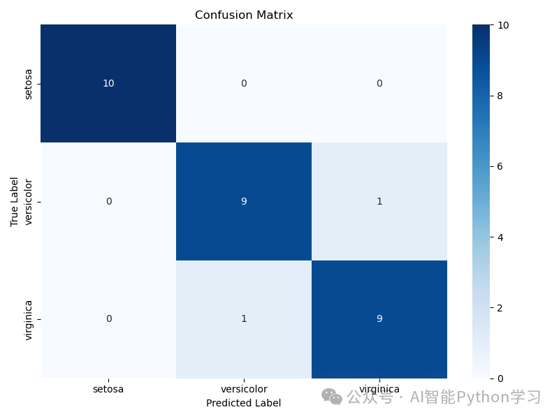

Visualization Section

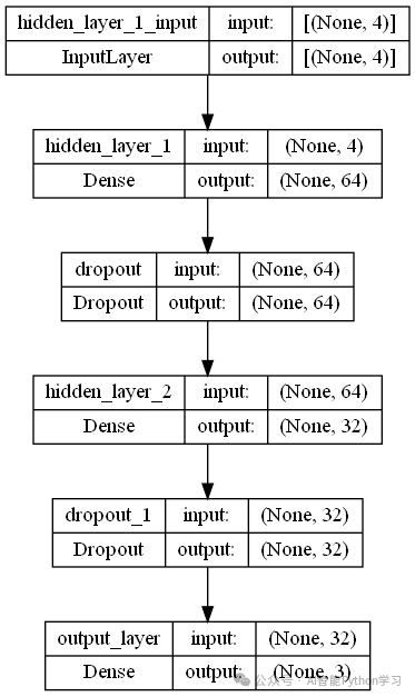
6.1 Draw Model Structure Diagram

# Draw model structure diagram and save
plot_model(model,
            to_file='mlp_iris_model.png',
            show_shapes=True,
            show_layer_names=True,
           dpi=96,
           rankdir='LR') # 'LR' means left to right, 'TB' means top to bottom
# You can also display directly in Notebook
# plot_model(model, show_shapes=True, show_layer_names=True)

6.2 Plot Loss and Accuracy Curves During Training

# Extract data from history object
history_dict = history.history
loss_values = history_dict['loss']
val_loss_values = history_dict['val_loss']
acc_values = history_dict['accuracy']
val_acc_values = history_dict['val_accuracy']
epochs = range(1, len(loss_values) + 1)

# Create canvas
fig, (ax1, ax2) = plt.subplots(1, 2, figsize=(16, 5))

# Plot loss curve
ax1.plot(epochs, loss_values, 'bo-', label='Training Loss')
ax1.plot(epochs, val_loss_values, 'ro-', label='Validation Loss')
ax1.set_title('Training and Validation Loss')
ax1.set_xlabel('Epochs')
ax1.set_ylabel('Loss')
ax1.legend()
ax1.grid(True)

# Plot accuracy curve
ax2.plot(epochs, acc_values, 'bo-', label='Training Accuracy')
ax2.plot(epochs, val_acc_values, 'ro-', label='Validation Accuracy')
ax2.set_title('Training and Validation Accuracy')
ax2.set_xlabel('Epochs')
ax2.set_ylabel('Accuracy')
ax2.legend()
ax2.grid(True)
plt.tight_layout()
plt.show()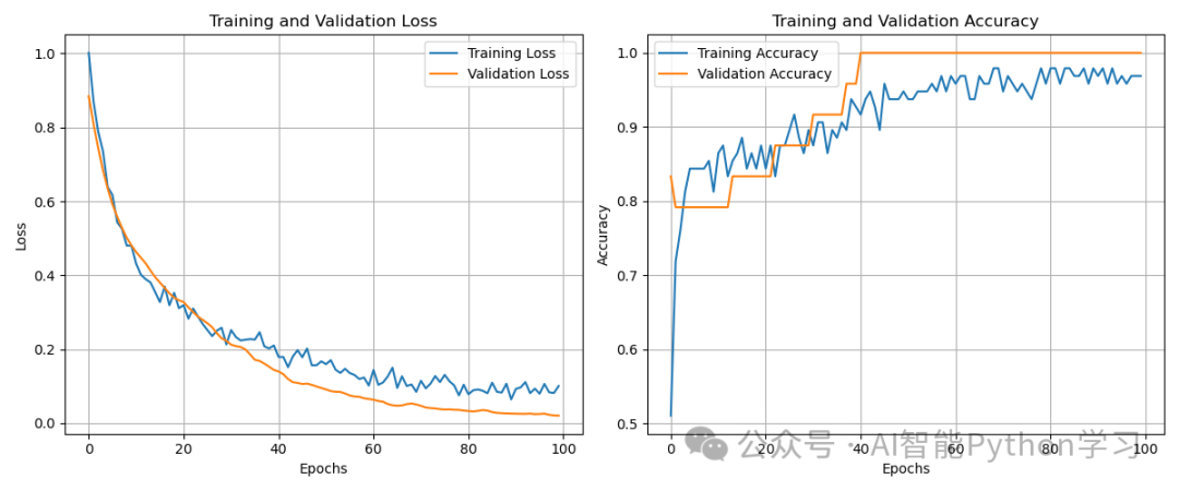

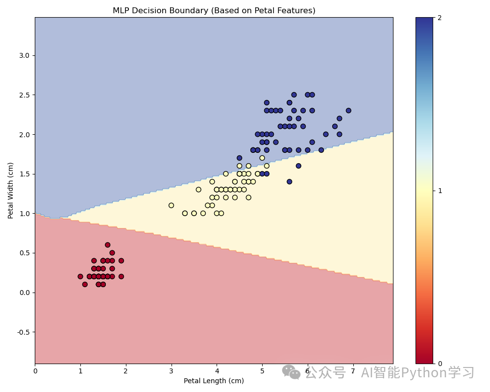
6.3 Plot Decision Boundaries (Select Two Features for Visualization)

Since the original data has 4 features, we select the two most important features to visualize the decision boundaries.

# Select two features: petal length and petal width
X_2d = X[:, 2:4] # Only take the last two features
X_train_2d, X_test_2d, y_train_2d, y_test_2d = train_test_split(
    X_2d, y, test_size=0.2, random_state=42, stratify=y)

# Retrain a simple model for visualization
model_2d = Sequential([
    layers.Dense(32, activation='relu', input_shape=(2,)),
    layers.Dense(16, activation='relu'),
    layers.Dense(3, activation='softmax')
])
model_2d.compile(optimizer='adam', loss='sparse_categorical_crossentropy', metrics=['accuracy'])
model_2d.fit(X_train_2d, y_train_2d, epochs=100, verbose=0)

# Create grid points
x_min, x_max = X_2d[:, 0].min() - 1, X_2d[:, 0].max() + 1
y_min, y_max = X_2d[:, 1].min() - 1, X_2d[:, 1].max() + 1
xx, yy = np.meshgrid(np.arange(x_min, x_max, 0.02),
                     np.arange(y_min, y_max, 0.02))

# Make predictions on grid points
Z = model_2d.predict(np.c_[xx.ravel(), yy.ravel()])
Z = np.argmax(Z, axis=1)
Z = Z.reshape(xx.shape)

# Plot decision boundaries
plt.figure(figsize=(10, 8))
plt.contourf(xx, yy, Z, alpha=0.4, cmap=plt.cm.RdYlBu)
scatter = plt.scatter(X_2d[:, 0], X_2d[:, 1], c=y, s=50, edgecolor='k', cmap=plt.cm.RdYlBu)
plt.xlabel('Petal Length (cm)')
plt.ylabel('Petal Width (cm)')
plt.title('MLP Decision Boundaries (Based on Petal Length and Width)')
plt.colorbar(scatter, ticks=[0, 1, 2], label='Class')
plt.show()