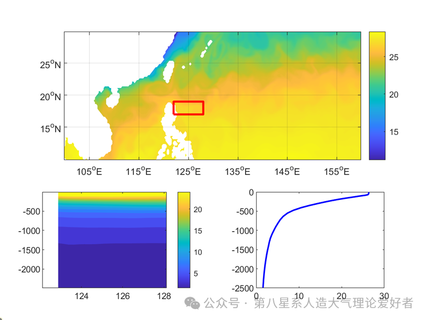
MATLAB Visualization of Sea Surface Temperature (SST) and Temperature Distribution in a Specified Marine Area
Author: The Eighth Galaxy – Xiang Xianjun
Email: [email protected]
close all
clear;
clc
%% First Figure - Plotting Sea Surface Temperature (SST) in a Specified Marine Area
load("D:\matlab2022\toolbox\T.mat") % Import data
figure
set(gcf,'Color','w')   % gcf is the figure handle, set the figure background color to white
% Extract the required longitude and latitude range
lon1=lon(400:640);
lat1=lat(400:480);
t=squeeze(T(1, 400:480, 400:640));     % Data dimensionality reduction
subplot("Position",[0.150.50.80.4]) % Modify subplot position attributes
% Plot 2D contour map
contourf(lon1,lat1,t,'k-','levellist',25,'LineWidth',1.0)
contourf(lon1,lat1,t,'levellist',0:0.1:30,'LineStyle','none')
hold on
% Rectangle annotation for the specified marine area
x1 = [122, 128, 128, 122, 122];
y1 = [17, 17, 19, 19, 17];
plot(x1,y1,'r-','LineWidth',2)
hold on
% gca is the coordinate handle, set the coordinate tick attributes
set(gca,'XTick',105:10:155, 'xticklabel',{'105^oE','115^oE',...'125^oE','135^oE','145^oE','155^oE'},'Ytick',15:5:25,...'yticklabel',{'15^oN','20^oN','25^oN'})
% h1 is the color bar handle, set the color bar attributes
h1 = colorbar;
set(h1,"Direction",'normal')
hold on
grid on  % Draw grid
%% Second Figure - Average Temperature Distribution in the Upper 2500 Meters within the Rectangular Marine Area
subplot("Position",[0.10.10.40.3])% Extract the required three-dimensional range
depth=depth(1:40);
lat2=lat(429:436);
lon2=lon(489:513);
t1=squeeze(mean(T(1:40, 429:436, 489:513),2));  % Data dimensionality reduction
set(gcf,'Color','w')  % gcf is the figure handle, set the figure background color to white
contourf(lon2,-depth,t1,'levellist',0:1.5:25,'LineStyle','none')
% Set h1 as the color bar handle, set the color bar attributes
h2 = colorbar;
set(h2,'YDir','normal')
%% Third Figure - Plotting the Vertical Distribution of Average Temperature within the Rectangular Marine Area
subplot("Position",[0.60.10.30.3])
t2=squeeze(nanmean(t1,2));   % Data dimensionality reduction
plot(t2,-depth,'b-','LineWidth',1.5)


END
Reply with ‘The Eighth Galaxy’ to join the group
Article edited by | Xiao Shiyi