Wind Power Generation Forecasting Based on GRU Optimized by Sparrow Algorithm

1. GRU Principles

RNNs are suitable for analyzing and processing time series data because they introduce a recurrent unit structure in the network, allowing internal connections between hidden units, which makes it possible to explore temporal relationships between non-continuous data. However, RNNs suffer from the vanishing gradient problem, which leads to a loss of the ability to learn information from the distant past as the time interval increases.

The introduction of LSTM neural networks addresses the vanishing gradient problem of RNNs and has been widely applied in the field of time series data prediction. In recent years, many variants have evolved based on different needs. GRU, as a variant of LSTM, adopts a gated recurrent neural network structure, requiring fewer training parameters while maintaining the predictive performance of LSTM. The internal units of GRU are quite similar to those of LSTM, with the difference being that GRU combines the input gate and forget gate of LSTM into a single update gate. Therefore, GRU has only two gate structures: the update gate and the reset gate. The update gate controls the extent to which the previous state information is retained in the current state; a larger value of the update gate indicates that more information from the previous state is retained. The reset gate determines whether to combine the current state with previous information; a smaller value of the reset gate indicates that more information is ignored.

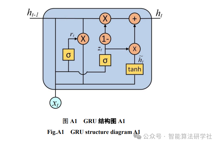
As mentioned earlier, let be the input, be the output of the hidden layer, and the GRU unit is calculated using the following formulas:

Where: and are the update gate and reset gate, respectively; is the summary of the input and the previous hidden layer output; is the Sigmoid function; is the hyperbolic tangent function; and are the training parameter matrices; represents the composite relationship of and .

2. Wind Power Forecasting

2.1 Dataset

The dataset consists of wind power data from 2019, as shown below:

Time	Wind Speed at 10m (m/s)	Wind Speed at 30m (m/s)	Wind Speed at 50m (m/s)	Wind Speed at 70m (m/s)	Hub Height Wind Speed (m/s)	Wind Direction at 10m (°)	Wind Direction at 30m (°)	Wind Direction at 50m (°)	Wind Direction at 70m (°)	Hub Height Wind Direction (°)	Temperature (°)	Pressure (hPa)	Humidity (%)	Actual Power Generation (MW)
2019-01-01 00:00:00	0.223	0	0	0.818	0.818	166.816	177.355	6.224	210.836	210.836	-13.154	898.71	53.497	0.979591

Excluding time, the data features consist of a total of 14 dimensions.

We use a window size of 5 days of data to predict the next day’s data, resulting in a total of 14*5=70 dimensions, with the output being 1-dimensional data, i.e., actual power generation (MW). In practical applications, the window size can be adjusted based on actual conditions.

3. GRU Optimized by Sparrow Algorithm

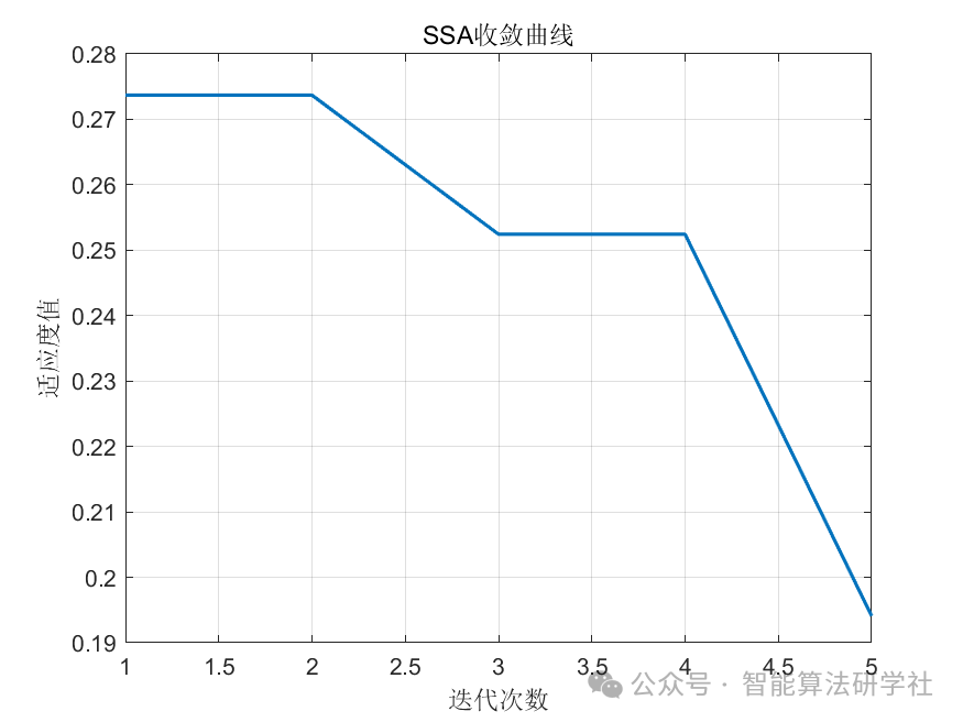
For the principle of the Sparrow Algorithm, please refer to: https://blog.csdn.net/u011835903/article/details/108830958 As mentioned earlier, the parameter settings of GRU are extensive. This paper utilizes the Sparrow Algorithm to optimize the parameters of LSTM (learning rate, number of GRU neurons, regularization parameter). The fitness function is designed as the average percentage error (MAPE) of the training set:

The fitness function selects the MAPE error after training. A smaller MAPE error indicates a higher degree of overlap between the predicted data and the original data. The final optimized output includes the best learning rate, number of GRU neurons, and regularization parameter. Then, the trained network with the best learning rate, number of GRU neurons, and regularization parameter is tested on the test dataset.

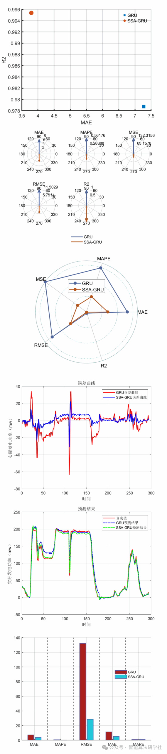
4. Experimental Results

5. Matlab Code

Click “Read the original text” to get it!!