The Fourier analysis of signals includes the Fourier transform of continuous signals and the Fourier transform of discrete signals.
Fourier Transform of Continuous Signals
Definition
Let x(t) be a continuous-time signal. If x(t) is absolutely integrable, that is,
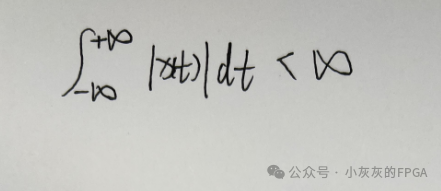
then the Fourier transform of x(t) exists and is defined as
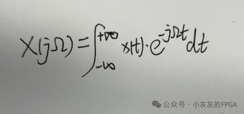
Its inverse transform is
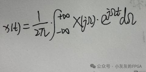
In the above equations, Ω=2πf, with units of rad/s. X(JΩ)=|X(JΩ)|e^(Jφ(Ω)), where |X(JΩ)| represents the amplitude-frequency characteristic, and φ(Ω) represents the phase-frequency characteristic.
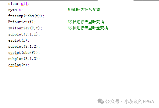
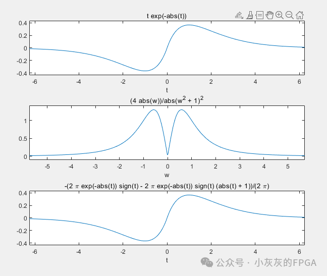
fourier and ifourier Functions
Matlab provides functions for calculating the Fourier transform and its inverse transform.
F=fourier(f) represents the Fourier transform of function f, returning a function of ω.
f=ifourier(F) represents the inverse transform of function F, with the default independent variable being ω, returning a function of x.
Before using the fourier and ifourier functions, the variables must be defined using the syms command. The returned functions are still symbolic variables, so use ezplot for plotting.
Fourier Series
Only non-periodic signals have Fourier transforms. If x(t) satisfies the Dirichlet conditions, it can be expanded into a Fourier series,
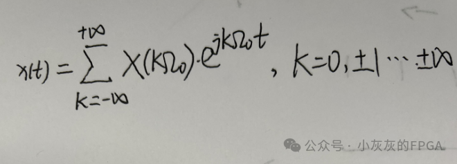
where Ω0=2πf0 represents the fundamental frequency of the signal x(t);
kΩ0 is the frequency of the k-th harmonic;
X(kΩ0) represents the Fourier series of x(t) at the k-th harmonic, with the amplitude indicating the magnitude of the frequency component kΩ0 contained in the signal x(t).
The periodic signal x(t) can be composed of an infinite number of complex sinusoids {e^(jkΩ0t), k=0,±1,…,±∞} multiplied by different weighting values X(kΩ0). X(kΩ0) is the amplitude of the corresponding complex sinusoid at frequency kΩ0.
X(kΩ0) takes values only at k=0,±1,…,±∞, thus it is discrete on the frequency axis,
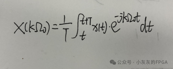
X(kΩ0) is represented in complex form as
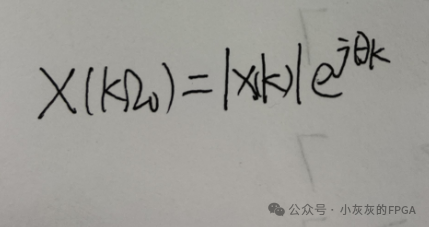
|X(k)| represents the amplitude of the component at frequency nf0;
θk represents the phase of the component at frequency nf0.
X(kΩ0) and X(jΩ)
X(kΩ0) is a discrete function on the Ω axis, taking integer multiples of Ω;
X(jΩ) is a continuous function of Ω.
X(kΩ0) represents the harmonic amplitudes;
X(jΩ) represents the spectral density.
Matlab Source Code
clear all;
n=0:30;
x=sin(0.2*n).*exp(-0.1*n);
k=0:30;
N=31;
X=x*(exp(-j*2*pi/N).^(n'*k));
subplot(2,1,1);
stem(n,x);
title('x sequence');
subplot(2,1,2);
stem(-15:15,[abs(17:end)abs(]);
title('X amplitude');