Color images (RGB), also known as true color images, are typically represented by three color components: red (R), green (G), and blue (B), with values ranging from [0,255].
Taking the reading, assignment, and display of a 24-bit true color image as an example, including matrix representation, matrix assignment, value retrieval, and single (color) channel display.
1. Matrix Representation of Color Images
Typically, a 24-bit image is represented as a three-channel data matrix, with data dimensions as follows: A simple example code is as follows:
I = imread('filename.bmp');         % I is an m×n×3 data matrix
imshow(I)                           % Display image I
imwrite(I,'newfilename.jpg','JPG'); % Save image I as another filename (newfilename.jpg) or format type (JPG,GIF,PNG,TIF, etc.)
1. Image Assignment and Retrieval
The example includes overall assignment and retrieval of the image, local area and single pixel data, and representation of single channel color components.
F = I;                % Overall assignment
s = I(10,20,:);       % Single pixel assignment
F = I(r1:r2,c1:c2,:); % Local data retrieval, r1 and r2 represent the starting and ending rows; c1 and c2 represent the starting and ending columns
Ir = I(:,:,1);        % Red component
Ig = I(:,:,2);        % Green component
Ib = I(:,:,3);        % Blue component
2. Displaying Single Color Images
If you need to display the red (R) component, you can set the green (G) and blue (B) components to zero, keeping only the red component.
F(:,:,2) = 0;         % Set green to 0
F(:,:,3) = 0;         % Set blue to 0
imshow(F);            % Red component
2. Grayscale Conversion of Images
Grayscale conversion of color images essentially extracts the brightness information from the color image. There are generally two methods to achieve grayscale conversion.
1. Using Brightness Equation
PAL Standard
Using the PAL standard brightness equation to extract brightness information. The specific code is as follows:
L = 0.222*Ir+0.707*Ig+0.071*Ib;   % R, G, B represent the grayscale values of the red, green, and blue channels of the color image. "*" indicates multiplication; the sum of the weight coefficients is 1
imshow(L,[])                      % Display grayscale image L, brackets [] for automatic adjustment of grayscale display
NTSC Standard
Using the NTSC standard brightness equation to extract brightness information. The specific code is as follows:
L = 0.229*Ir+ 0.587*Ig+ 0.114*Ib; % The variable meanings are the same as above, the sum of the weight coefficients is 1
HSV/HSI Conversion
Conversion from RGB color space to HSV and HSI color space. The specific code is as follows:
Ihsv = rgb2hsv(I); % RGB to HSV
V = Ihsv(:,:,3);   % Maximum value among the red, green, and blue components of a specific color
H and S represent hue and saturation, respectively.
2. Built-in MATLAB Function for Grayscale Conversion
The specific code is as follows:
L = rgb2gray(I); % Grayscale processing of color images (NTSC)
In fact, the built-in MATLAB function rgb2gray utilizes the NTSC standard brightness equation for grayscale processing of color images.
3. Example Code
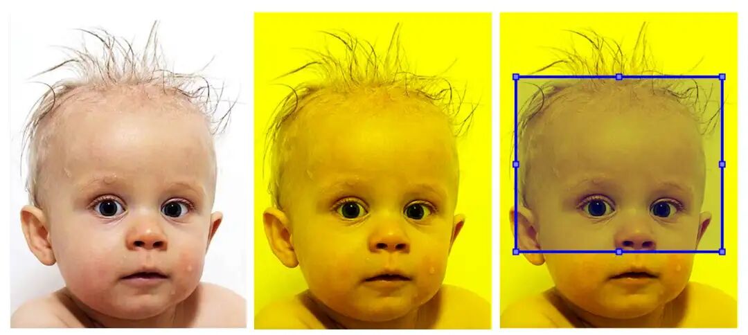
The following code mainly implements single component display and local image display through mouse selection.
%==========================================================================
% DEMO: Understanding Color Images
%    Name: SEERGBIMAGE
%    Course:  Digital Image Processing(DIP)
%
%    Copyright (c) 2006-2025 Zhenming Peng
%    IDIPLAB,
%    School of Information and communication engineering,
%    University of Electronic Science and Technology of China
%    http://idiplab.uestc.cn/
%
%    Revised: 2025.09.02
% See Also RGB2GRY, CAT, DRAWRECTANGLE
%==========================================================================
clc, clear, close all;

I = imread('.\data\boy.jpg');

imshow(I),title('The original image','FontSize',12)

if ndims(I)~=3   % or size(I,3)~=3
   disp('Must be a color image')
   return,
end

Ir = I(:,:,1);          % Red component R
Ig = I(:,:,2);          % Green component G
Ib = I(:,:,3);          % Blue component B

J = I;                  % Matrix assignment (global)
% J = cat(3,Ir,Ig,Ib);  % Concatenate arrays

% J(:,:,1) = 0;         % Set R component to 0
% J(:,:,2) = 0;         % Set G component to 0
J(:,:,3) = 0;           % Set B component to 0

% Brightness equation (亮度方程)
% L = 0.222R+0.707G+0.071B (PAL 制式)
% L = 0.299R+0.587G+0.114B (NTSC制式)

% Convert RGB image or colormap to grayscale
Igray = 0.299*Ir+0.587*Ig+0.114*Ib;
% Igray = rgb2gray(I);

figure;
imshow(J),title('Single color channel','FontSize',12)

[rows, cols, ~] = size(I);  % Array size

% Mouse capture of local region of interest (ROI)
ax = gca;
roi = drawrectangle(ax,'Color','b');   % Draw a rectangle as ROI
if ishandle(ax)
    pos = round(roi.Position);
    width = pos(1)+pos(3);
    width(width>cols) = cols;          % Limit columns beyond boundaries
    height = pos(2)+pos(4);
    height(height>rows) = rows;        % Limit rows beyond boundaries
else
    disp('The current figure is closed')
    return
end

% Local area (ROI) display
% imRoi = Igray(pos(2):height, pos(1):width);  % graylevel image
imRoi = J(pos(2):height, pos(1):width,:);      % RGB image
figure;
imshow(imRoi),title('The ROI image','FontSize',12)
The code execution result is as follows:
“The true luxury is having the switch to turn off the noisy world in your hands!”

Text and images: Zhenming Peng
Editor: Simin LiuPreviousIssuesReview
MATLAB Image Processing | Constructing Frequency Domain Filters from Spatial Domain Templates (Complete Code Included)
MATLAB Plotting Techniques | Setting Transparency of Color Bars (Complete Code Included)
MATLAB Plotting Techniques | Capturing Frames to Generate GIF Animations (Complete Code Included)
MATLAB Plotting Techniques | Standard Labeling of Graphics (With Example Code)
MATLAB Signal Simulation | Understanding Frequency Resolution of Fourier Transform (With Example Code)
MATLAB Image Processing | Homomorphic Filtering of Grayscale Images (Complete Code Included)
MATLAB Plotting Techniques | Drawing Dual Y-Axis Line Charts (With Example Code)
MATLAB Image Processing | Sigmoid Function Contrast Stretching (With Example Code)
MATLAB Plotting Techniques | Gamma Transformation Curve of Image Grayscale (With Example Code)
MATLAB Plotting Techniques | Clever Use of Graphics Handles (With Example Code)
MATLAB Plotting Techniques | Area Filling Between Two Lines with Color (With Source Code)
MATLAB Plotting Techniques | 3D Visualization Code Optimization of Fourier Series Expansion
MATLAB Plotting Techniques | Data Visualization Color Schemes (With Code)
MATLAB Plotting Techniques | Pseudocolorization of Grayscale Images (With Code)
MATLAB Plotting Techniques | Density Scatter Plot + Regression Line Removal (With Code)
MATLAB Plotting Techniques | 2D Scatter Plot (With Code)
MATLAB Plotting Techniques | 3D Curve Filling (With Code)
MATLAB Plotting Techniques | 3D Line Chart (With Code)
MATLAB Plotting Techniques | 3D Surface (With Code)
MATLAB Plotting Techniques | Homemade Music Player (With Code)
MATLAB Plotting Techniques | Polygon Area Filling Graph (With Code)
MATLAB Plotting Techniques | Drawing Color Gradient Line Charts (With Code)
MATLAB Plotting Techniques | Line Chart Drawing (With Code)
MATLAB Plotting Techniques | Drawing Color Gradient Bar Charts
What moves you is not someone else’s story, but the shadow of yourself read from someone else’s story.