Click the "Xiaobai Learns Vision" above, select "Star" or "Top"
Important content delivered at the first time
Introduction
In yesterday’s article, we introduced histogram processing based on grayscale images and briefly mentioned histogram processing of color images, but did not discuss the best methods.
Let’s start by importing all the necessary libraries!
import numpy as np
import matplotlib.pyplot as plt
from skimage.io import imread, imshow
import matplotlib.pyplot as plt
from skimage.exposure import histogram, cumulative_distribution
from scipy.stats import norm
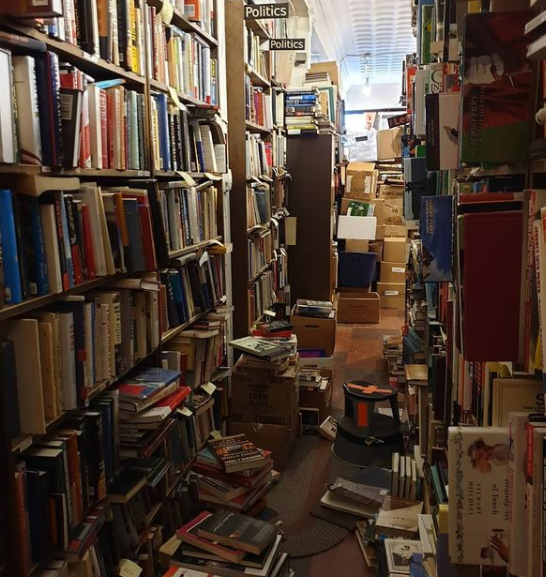
Now let’s load the image.
dark_image = imread('dark_books.png');
plt.figure(num=None, figsize=(8, 6), dpi=80)
imshow(dark_image);
To help us better understand the RGB layers in this image, let’s isolate each individual channel.
def rgb_splitter(image):
    rgb_list = ['Reds','Greens','Blues']
    fig, ax = plt.subplots(1, 3, figsize=(17,7), sharey = True)
    for i in range(3):
        ax[i].imshow(image[:,:,i], cmap = rgb_list[i])
        ax[i].set_title(rgb_list[i], fontsize = 22)
        ax[i].axis('off')
    fig.tight_layout()
rgb_splitter(dark_image)
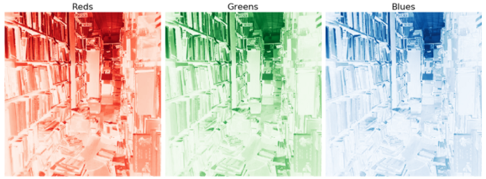
Now that we have a general understanding of the individual color channels, let’s take a look at their CDF.
def df_plotter(image):
    freq_bins = [cumulative_distribution(image[:,:,i]) for i in range(3)]
    target_bins = np.arange(255)
    target_freq = np.linspace(0, 1, len(target_bins))
    names = ['Red', 'Green', 'Blue']
    line_color = ['red','green','blue']
    f_size = 20
    fig, ax = plt.subplots(1, 3, figsize=(17,5))
    for n, ax in enumerate(ax.flatten()):
        ax.set_title(f'{names[n]}', fontsize = f_size)
        ax.step(freq_bins[n][1], freq_bins[n][0], c=line_color[n], label='Actual CDF')
        ax.plot(target_bins, target_freq, c='gray', label='Target CDF', linestyle = '--')
df_plotter(dark_image)
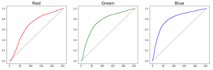
As we can see, all three channels are quite far from the ideal straight line. To address this issue, let’s simply interpolate their CDF.
def rgb_adjuster_lin(image):
    target_bins = np.arange(255)
    target_freq = np.linspace(0, 1, len(target_bins))
    freq_bins = [cumulative_distribution(image[:,:,i]) for i in range(3)]
    names = ['Reds', 'Blues', 'Greens']
    line_color = ['red','green','blue']
    adjusted_figures = []
    f_size = 20
    fig, ax = plt.subplots(1,3, figsize=[15,5])
    for n, ax in enumerate(ax.flatten()):
        interpolation = np.interp(freq_bins[n][0], target_freq, target_bins)
        adjusted_image = img_as_ubyte(interpolation[image[:,:,n]].astype(int))
        ax.set_title(f'{names[n]}', fontsize = f_size)
        ax.imshow(adjusted_image, cmap = names[n])
        adjusted_figures.append([adjusted_image])
    fig.tight_layout()
    fig, ax = plt.subplots(1,3, figsize=[15,5])
    for n, ax in enumerate(ax.flatten()):
        interpolation = np.interp(freq_bins[n][0], target_freq, target_bins)
        adjusted_image = img_as_ubyte(interpolation[image[:,:,n]].astype(int))
        freq_adj, bins_adj = cumulative_distribution(adjusted_image)
        ax.set_title(f'{names[n]}', fontsize = f_size)
        ax.step(bins_adj, freq_adj, c=line_color[n], label='Actual CDF')
        ax.plot(target_bins, target_freq, c='gray', label='Target CDF', linestyle = '--')
    fig.tight_layout()
    return adjusted_figures
channel_figures = return adjusted_figures
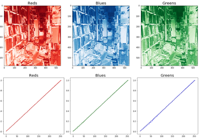
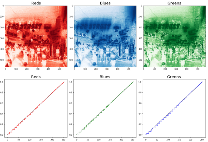
We see significant improvements in each color channel.
Additionally, note how the function above returns all these values as a list. This will help us in our final step to recombine all of these into a single image. To better understand how to do this, let’s check our list.
print(channel_figures)
print(f'Total Inner Lists : {len(channel_figures)}')
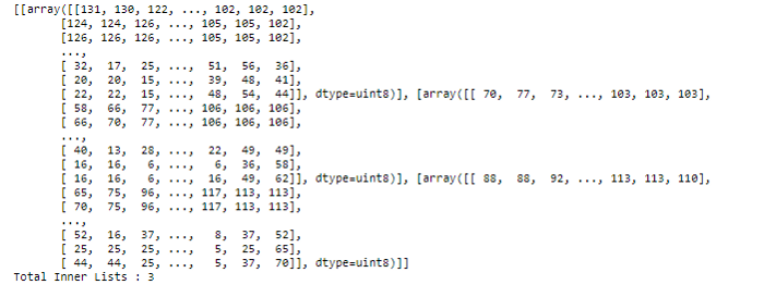
We see that there are three lists in the variable channel_figures. These lists represent the values of the RGB channels. Below, we can recombine all these values together.
plt.figure(num=None, figsize=(10, 8), dpi=80)
imshow(np.dstack((channel_figures[0][0], channel_figures[1][0], channel_figures[2][0])));
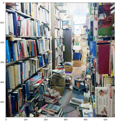
Notice how significant the difference is before and after image processing. The image not only brightened significantly, but the yellowish tint was also removed. Let’s try the same processing on a different image.
dark_street = imread('dark_street.png');
plt.figure(num=None, figsize=(8, 6), dpi=80)
imshow(dark_street);
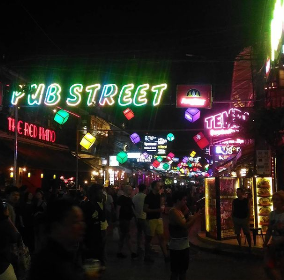
Now that we have loaded a new image, let’s process it simply using the function.
channel_figures_street = adjusted_image_data = rgb_adjuster_lin(dark_street)
plt.figure(num=None, figsize=(10, 8), dpi=80)
imshow(np.dstack((channel_figures_street [0][0], channel_figures_street [1][0], channel_figures_street [2][0])));
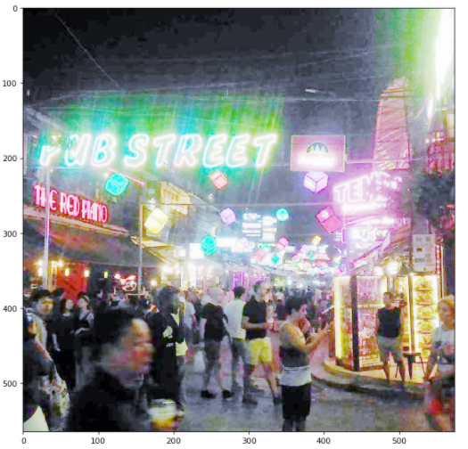
We can see the amazing changes. It is undeniable that this photo is a bit overexposed. This may be due to the obvious neon lights in the background. In future articles, we will learn how to fine-tune our approach to make our functions more general.
Conclusion
In this article, we learned how to adjust each RGB channel to retain the color information of the image. This technique is a significant improvement over previous grayscale adjustment methods.
Download 1: OpenCV-Contrib Extension Module Chinese TutorialReply to “Xiaobai Learns Vision” in the public account backend:Chinese Tutorial for Extension Modules, you can download the first Chinese version of the OpenCV extension module tutorial online, covering installation of extension modules, SFM algorithms, stereo vision, target tracking, biological vision, super-resolution processing and more than twenty chapters.Download 2: 31 Lectures on Python Vision Practical ProjectsReply to “Python Vision Practical Projects 31 Lectures” in the public account backend:Python Vision Practical Projects 31 Lectures, you can download 31 practical vision projects including image segmentation, mask detection, lane line detection, vehicle counting, eyeliner addition, license plate recognition, character recognition, emotion detection, text content extraction, facial recognition to help quickly learn computer vision.Download 3: 20 Lectures on OpenCV Practical ProjectsReply to “OpenCV Practical Projects 20 Lectures” in the public account backend:, you can download 20 practical projects based on OpenCV to achieve advanced learning of OpenCV.Download 4: Leetcode Algorithm Open Source BookReply to “leetcode” in the public account backend:, you can download.Every question beats 100% runtime, an open-source book you deserve to own!
Discussion Group
Welcome to join the reader group of the public account to communicate with peers. Currently, there are WeChat groups for SLAM, three-dimensional vision, sensors, autonomous driving, computational photography, detection, segmentation, recognition, medical imaging, GAN, algorithm competitions etc. (which will be gradually subdivided), please scan the WeChat number below to join the group, and note: “nickname + school/company + research direction”, for example: “Zhang San + Shanghai Jiaotong University + Visual SLAM”. Please note according to the format, otherwise it will not be approved. After successfully adding, you will be invited to enter the relevant WeChat group based on your research direction. Please do not send advertisements in the group, otherwise you will be removed from the group, thank you for understanding~