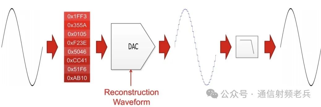
First, what is a Digital-to-Analog Converter (DAC)? A DAC is used to convert digital samples in bit form into analog waveforms of current or voltage. In short, a DAC is used to reconstruct an analog signal from a digital signal. The process of reconstructing an analog signal from a digital signal is as follows.
First, a series of digital samples representing the desired analog signal is input into the DAC. Next, the DAC outputs the digital samples by using a reconstructed waveform weighted by the digital samples, thereby performing analog reconstruction. Finally, an analog filter is used to smooth the output response. The analog filter is used to remove unwanted signals (called mirror signals) from the output signal.
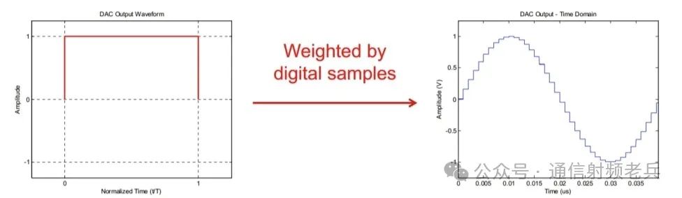
The reconstructed waveform determines the output response of the Digital-to-Analog Converter (DAC) in both the time and frequency domains. At each sampling moment, the DAC outputs a reconstructed waveform weighted by the digital samples. The left side of the figure below shows an example of a rectangular reconstructed waveform. This waveform has a constant amplitude during the sample duration (from time 0 to T) and is zero elsewhere.
This waveform holds the sample value constant during the sample clock period, commonly referred to as a Zero-Order Hold (ZOH) waveform. We will discuss this in more detail later.
The right side of the figure below shows a sine wave output from the DAC using this reconstructed waveform. Note its stepped response. The selected reconstructed waveform also results in a certain frequency response.
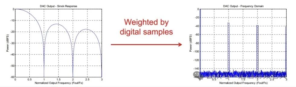
The frequency response determines the output power of the desired signal and the power of the unwanted mirror signals. The left side of the figure below shows the frequency response of the rectangular or Zero-Order Hold waveform from the previous figure (for frequencies from DC to three times the sampling rate). We can see that it exhibits characteristics similar to the sinc function or sin(x)/x response, with power levels decreasing at higher output frequencies.
The right side of the figure below displays the frequency domain representation of the DAC output of the sine wave after reconstruction from the previous figure. We can see multiple tones at different output power levels in the response. The power of these tones corresponds to the frequency response of the reconstructed waveform shown on the left.
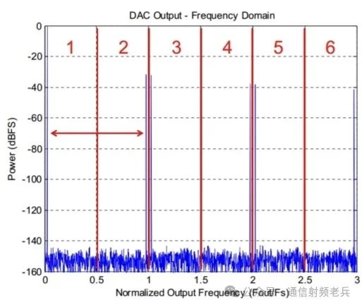
Before continuing, let’s take a moment to define the Nyquist zone. The Nyquist zone defines a frequency bandwidth that is half the sampling frequency. The first Nyquist zone starts from 0 Hz (or DC) and extends to half the sampling frequency FS (FS/2), where FS is the sampling rate of the DAC. The second Nyquist zone extends from half of FS to FS, and so on. Here, we highlight the first six Nyquist zones. Note that the spectral characteristics of even-numbered Nyquist zones are mirrored compared to the odd-numbered zones, so in the second Nyquist zone, the low frequencies correspond to high frequencies from the first Nyquist zone.
Mirror spectra can be seen in the second, fourth, and sixth Nyquist zones. The output power in each Nyquist zone depends on the frequency response of the reconstructed waveform, as shown in the figure above. The Nyquist zones are named after the Nyquist sampling theorem.
The first Nyquist zone represents the basic definition of the Nyquist sampling theorem, which states that the sampling rate must be twice the highest output frequency, while the other Nyquist zones represent the extension of the bandpass signal sampling theorem. Most DACs are designed to operate only within the first Nyquist zone, but some can operate in higher Nyquist zones. We will discuss DACs that support multiple Nyquist zones in more detail later.
Having understood the above, let’s take a closer look at the non-ideal DAC output response. In the third figure, we can see that the frequency response is not completely flat in the first Nyquist zone. At the end of the first Nyquist zone, the output power decreases by 4 dB. Typically, the response is flattened by using a digital filter to inverse the response.
The fourth figure shows the mirroring that occurs in other Nyquist zones when the signal is reconstructed. In this case, the desired signal is a low-frequency sine wave within the first Nyquist zone. However, we also see sine waves near FS, 2×FS, and 3×FS.
These are the mirrors that appear within each Nyquist zone due to the non-ideal reconstructed waveform.
Each Nyquist zone will have a mirror. Since we have displayed six Nyquist zones, we see six mirrors, including the expected mirror within the first Nyquist zone. Filters are needed to remove the unwanted mirrors.