Introduction to AdaLoRA: Adaptive Weight Matrix Fine-Tuning for Large Models

Introduction: AdaLoRA addresses the issue of manually selecting the low-rank parameter r in LoRA and implements dynamic adjustments to all key parts of the model (including FFN), comprehensively enhancing model capabilities.

Issues with LoRA

LoRA allows for the original model parameters to remain unchanged while training a “small patch” (low-rank matrix ΔW) that is added to the original model (W = W₀ + ΔW). This means only this small patch needs to be trained, significantly saving computational resources. However, there are issues that need to be resolved.

Fixed rank (r) is not flexible enough: LoRA requires you to decide in advance the complexity of this “small patch” (referred to as “rank r”). However, different layers and tasks require different complexities, and a uniform setting may either waste parameters or fail to fine-tune to achieve the best results. Uniformly allocating parameter budgets is unreasonable.
Only adjusting the Attention part while ignoring FFN (Feed-Forward Network): LoRA defaults to fine-tuning only the self-attention layers (Attention), but the feed-forward network (FFN) in the model is also very important, and ignoring it may limit the model’s performance.

Introduction to AdaLoRA

The core idea of AdaLoRA is:Intelligently and adaptively allocating parameter budgets, putting more parameters in “more important places” to solve the problems present in LoRA.

The specific implementation principles include:

Using SVD decomposition instead of low-rank matrices: AdaLoRA uses Singular Value Decomposition (SVD) to represent the incremental update ΔW. SVD is certainly better than manual methods; it can decompose a matrix into three parts: U Σ Vᵀ, where Σ is a diagonal matrix representing the importance of each dimension (the larger the singular value, the more important it is). This allows us to dynamically adjust each parameter based on importance. For more on SVD decomposition, see the introduction at the end of the article.
Importance scoring + dynamic pruning: AdaLoRA calculates an “importance score” for each parameter (or group of parameters) based on SVD singular values and gradient information during training, determining how much contribution it has to the new task. Like a gardener pruning branches: important ones are retained or even strengthened, while unimportant ones are pruned (parameters set to 0). This achievesdynamically allocating parameter budgets across different layers and modules, rather than a one-size-fits-all approach.
Simultaneously fine-tuning Attention and FFN: AdaLoRA no longer focuses solely on Attention but fine-tunes all key parts of the model (including FFN), comprehensively enhancing the model’s ability to adapt to new tasks.

A vivid metaphor: full parameter fine-tuning is like renovating an entire building, which is time-consuming and costly.LoRA applies the same wallpaper to every room, regardless of its purpose,AdaLoRA first assesses the importance of each room: using expensive wallpaper in the living room, waterproof paint in the bathroom, and simply painting the storage room white—saving money while achieving good results.

SVD Decomposition Instead of Low-Rank Matrices

1. Calculating Importance Scores

AdaLoRA models the importance of parameters and combines it with SVD decomposition. This process is the core of AdaLoRA’s intelligence compared to LoRA.

AdaLoRA believes that the importance of a parameter s(w) depends on two aspects:

Sensitivity I(w): How much does this parameter affect the final outcome? If it changes slightly, will the loss function change drastically?
Uncertainty U(w): How confident are we in our sensitivity assessment of this parameter? Is its value stable or fluctuating significantly?

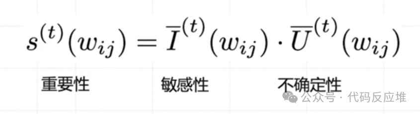
Sensitivity measures: how much changing this parameter will affect the model’s loss function.: Sensitivity ≈ weight value * gradient value. This is like evaluating an employee’s influence; you need to consider both their position and whether their work is on the critical path.

To prevent drastic fluctuations in sensitivity during training, AdaLoRA uses **moving averages** to smooth the sensitivity values of each round, making them more stable. Here, `β₁` is a hyperparameter (e.g., 0.99) used to control the weight of historical values.

Uncertainty measures: how confident we are in the sensitivity value calculated above. If a parameter’s sensitivity varies greatly in each training iteration, it indicates that our assessment is very unstable, leading to high uncertainty. If it is stable, uncertainty is low.

Finally, multiplying the smoothed sensitivity I(w) and uncertainty U(w) gives the final importance score for that parameter S(w).

2. Substituting Importance Scores into SVD

LoRA decomposes the incremental update ΔW into two small matrices B and A (ΔW = B A), optimizing them equally.

AdaLoRA is more refined; it uses the triplet from SVD instead of the pair from LoRA. It decomposes ΔW using SVD, and instead of treating all parameters from the SVD decomposition equally, it calculates a total importance score foreach SVD triplet** which consists of the following three parts:

Singular value λ itself’s importance score.This is the most important part**, as the singular value directly represents the importance of that dimension.
Average importance score of all parameters in the left singular vector P.
Average importance score of all parameters in the right singular vector Q.

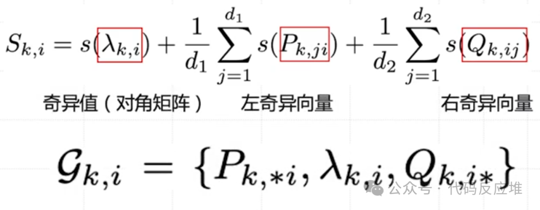
The purpose of this approach is: not only to look at whether the singular value λ itself is important, but also to see whether the vectors supporting this “important direction” P and Q are also important. This is a more comprehensive and robust assessment.

Dynamic Pruning Fine-Tuning

1. Setting Goals

AdaLoRA is not blindly optimizing; rather, it strives to reduce the model’s error while adhering to mathematical rules (maintaining matrix orthogonality)..

L(P, E, Q): is theobjective function for the entire optimization process, representing the “cost” or degree of “badness” of the model’s current state.
𝐶(𝑃,𝐸,𝑄): the main objective, minimizing model prediction loss. That is, theloss function Loss. This is a very standard concept in machine learning.
𝑅(𝑃𝑘,𝑄𝑘): the regularization term, ensuring the orthogonality of the left singular vector matrix P and the right singular vector matrix Q (team collaboration norms), aiming tomaintain numerical stability, ensuring the structural validity of SVD decomposition, thus making the importance scores and pruning operations more reliable.
𝛾: a hyperparameter controlling the weight of the regularization term. It is aweight coefficient. It controls the importance of the regularization term R relative to the main loss C.

If γ = 0, AdaLoRA completely ignores orthogonality, pursuing task performance, which may lead to training instability.
If γ is too large, AdaLoRA will overly emphasize maintaining orthogonality, potentially sacrificing task performance.
Therefore, γ needs an appropriate value to balance both.In simple terms:γ * Σ R(P_k, Q_k) answers the question—”Is the structure of the model parameters elegant and stable?”

2. Initial Training (Initial Phase)

In the initial phase, AdaLoRA is similar to LoRA, both training and updating parameters normally, that is, adjusting the resources allocated to them throughgradient descent (singular values Λ).

3. Model Pruning (Mid-Phase)

Calculating importance scoresS, assessing theimportance of the triplet (the size of the singular value λ),stability (uncertainty), andinfluence (sensitivity).

All triplets are sorted by score from highest to lowest.

When reaching time t, collect all importance scores, retaining only those ranked in the top `b^{(t)}`, while recycling resources from the others, completely removing the less important triplets (setting their singular value `λ` to 0). This is equivalent to reclaiming the parameter budget allocated to these directions and **redistributing**: reallocating the reclaimed budget to those with higher importance scores, even allowing important matrices to create new triplets (increasing rank `r`).

4. Stabilization Phase

The budget will be fixed at a lower level b^{(T)} for the final sprint and final fine-tuning. This is called the stabilization phase. Ensuring the model converges and stabilizes performance.

5. Budget Scheduling for Each Phase

Initial Phase (0≤𝑡<𝑡<ti): high budget 𝑏(0), extensive exploration.
Decay Phase (𝑡𝑖≤𝑡<T−tf): non-linear budget reduction, focusing on important directions, knowing which are important directions, gradually and non-linearly reducing the total budget, with increasing intensity of elimination, becoming more focused, adaptively adjusting rank r, increasing the values of the singular values corresponding to important directions λ. Since the singular values of unimportant directions are set to zero, theireffective “intrinsic rank” r is reduced; while the singular values of important directions become larger, theireffective “importance” increases. This achievesdynamically and adaptively allocating parameter budgets between different weight matrices.
Stabilization Phase (𝑡≥T−tf): fixed low budget b(T), final fine-tuning, ensuring model convergence and stable performance.

AdaLoRA Experimental Data

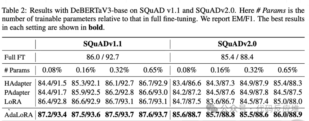
Task Description: SQuAD is a machine reading comprehension task where the model needs to answer questions based on the article. EM (Exact Match) and F1 scores are evaluation metrics, the higher the better.

Overwhelming Advantage: Under all parameter settings (0.08%, 0.16%, 0.32%, 0.65%), AdaLoRA’s EM and F1 scores comprehensively surpassed traditional full fine-tuning (Full FT) and other efficient fine-tuning methods (HAdapter, PAdapter, LoRA). This is an astonishing result in practice, indicating that better performance can be achieved with less than 1% of the parameters.
Comparison with LoRA: A direct comparison between AdaLoRA and LoRA shows a clear stability advantage for AdaLoRA. For example, on SQuADv1.1, even when AdaLoRA uses only 0.08% of the parameters (87.2/93.4), it significantly outperforms LoRA using 0.65% of the parameters (86.7/93.1). This proves thatadaptive parameter allocation is much more efficient than simple fixed-rank allocation.
Parameter Utilization Efficiency: For AdaLoRA, the performance improvement from increasing the parameter amount (from 0.08% to 0.65%) is very small, indicating that it is already close to its performance limit with an extremely low parameter count.Other methods (like LoRA) rely more on increasing the number of parameters to enhance performance.

Conclusion: In reading comprehension tasks, AdaLoRA achieves the best in both parameter efficiency and final results.

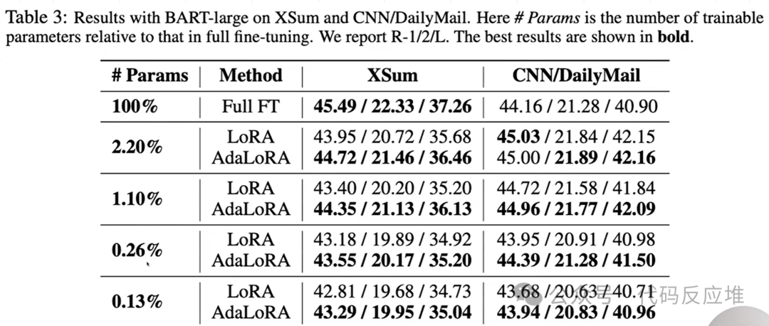
Task Description: The text summarization task requires the model to generate shorter, refined summaries. Using ROUGE-1, ROUGE-2, ROUGE-L as evaluation metrics, the higher the better.

Comprehensive Lead: In direct comparison with LoRA, AdaLoRA achieved higher ROUGE scores on almost all parameter settings and datasets. This proves that AdaLoRA’s advantagesare not limited to classification or reading comprehension tasks, but are equally effective in generative tasks.
Significant Advantage Under Low Budget: The fewer the parameters, the more pronounced AdaLoRA’s advantages often are. For example, on the XSum dataset, when the parameter count is only 0.13%, AdaLoRA’s ROUGE-L is 35.04, while LoRA’s is 34.73. This gap is a very valuable improvement in low-resource scenarios.
Surpassing Full Fine-Tuning: On the CNN/DailyMail dataset, AdaLoRA with only 2.2% parameters and LoRA has already surpassed full fine-tuning (44.16/21.28/40.90). This again highlights the enormous potential of parameter-efficient fine-tuning methods.

Conclusion: In the text summarization task, AdaLoRA also proves its outstanding effectiveness and parameter efficiency.

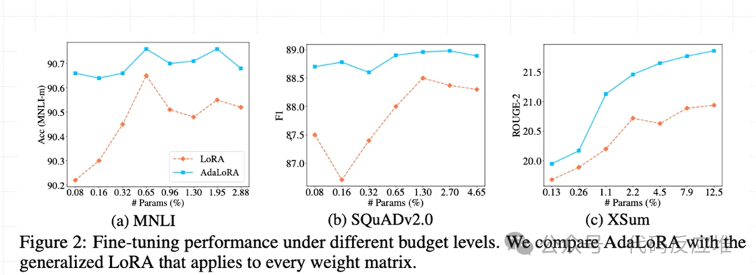
Chart Description: This curve shows the trend of model performance (accuracy/F1) as the number of trainable parameters (budget) increases.

Data Interpretation:

Global Advantage: AdaLoRA’s curve is always above LoRA’s curve. This means that at any budget level, choosing AdaLoRA will yield better performance than LoRA.
Marginal Benefits: It can be seen that both curves enter a “plateau” after a certain amount of parameters, where the benefits of increasing parameters diminish. However, AdaLoRA’s plateau comes earlier and is positioned higher. This indicates that AdaLoRA can achieve “saturated performance” with fewer parameters.
Greatest Gap Under Low Budget: On the far left, where the budget is very low, the gap between the two curves is the largest. This proves that AdaLoRA’sadaptive budget allocation strategy is most advantageous in scenarios with extremely limited parameters, as it ensures that every parameter is used effectively.

Conclusion: This graph intuitively demonstrates the comprehensive advantages of AdaLoRA over fixed-rank methods from a trend perspective.

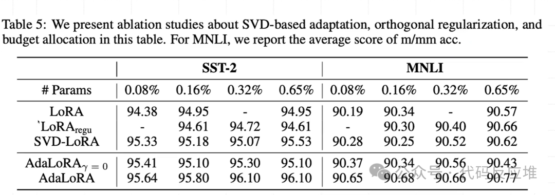
Experimental Description: Ablation experiments are conducted to verify whether each design component of AdaLoRA (SVD form, orthogonal constraints, dynamic budget allocation) is necessary and how much each contributes.

LoRA: The original LoRA method.
LoRAregu: Adding orthogonal constraints to LoRA.
SVD-LoRA: Using SVD form but without dynamic allocation (fixed rank).
AdaLoRA(γ=0): Using SVD form and dynamic allocation but removing orthogonal constraints.
AdaLoRA: The complete version of AdaLoRA.

Data Interpretation:

Importance of Orthogonal Constraints: Comparing AdaLoRA(γ=0) and AdaLoRA, it can be seen that adding orthogonal constraints (γ≠0) leads to stable performance improvements in most cases. This proves thatmaintaining the orthogonality of singular vectors is crucial for stability.
The Core Role of Dynamic Allocation: Comparing SVD-LoRA and AdaLoRA,AdaLoRA is significantly stronger. This indicates that merely using the SVD form (instead of BA) brings limited improvements; the real performance gain mainly comes from the dynamic budget allocation strategy.
The Power of Combination: The complete AdaLoRA is the best in almost all settings, indicating thatthe combination of SVD form, orthogonal constraints, and dynamic allocation is the optimal solution.

Conclusion: Ablation experiments confirm that every design in AdaLoRA is necessary, and they work together to achieve the best results.

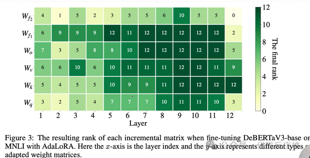
Chart Description: This heatmap shows the final rank (the darker the color, the higher the rank) allocated to different layers of the DeBERTa model (x-axis) and different weight matrices (y-axis) after fine-tuning.

Data Interpretation:

Dynamic Allocation vs. Average Allocation: AdaLoRA does not allocate the same rank to all matrices. For example, W_f1 and W_f2 (the two weight matrices of the FFN layer) receive higher average ranks, while W_q, W_k, W_v (the projection matrices of the attention layer) receive lower average ranks. This aligns with a general prior: FFN layers typically contain more task-specific knowledge than attention layers.
Inter-layer Differences: The same type of matrix is allocated different ranks across different layers. This indicates thatthe importance of different layers for downstream tasks indeed varies, and AdaLoRA successfully captures this difference.
Visual Verification: This figure providesdirect evidence of AdaLoRA’s core idea. It intuitively tells us that AdaLoRA has indeed learned the strategy of “putting good steel where it matters” in practice, rather than just in theory.

Conclusion: This graph empirically confirms that AdaLoRA can intelligently and adaptively allocate different importance (reflected as different ranks) to the incremental matrices.

Introduction to SVD Derivation

0. Introduction

Assuming we have two users (Alice, Bob) rating two movies (Wolf Warrior 1, Wolf Warrior 2), this can be viewed as dimensions.

The rating matrix A is a 2×2 matrix, thus an nxn matrix is also called a square matrix, and only square matrices can calculate eigenvalues. If it is an mxn matrix, SVD will decompose it into two square matrices mxm and nxn for calculation.

The following example explains based on an nxn square matrix.

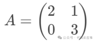
Using SVD to decompose the matrix A = U Σ Vᵀ. Analyzing this matrix: each row is equivalent to a data sample record, here there are two sample rows.

Imagine each value as the intensity value of a certain feature (movie) (how good it is), for example, 2 represents the attractiveness of Wolf Warrior 1 being 2.

1. Calculating Vᵀ (Right Singular Vector) (Right Singular Vector)

Meaning: A basic unit matrix on the minimum unit in the column space coordinate system.

Calculating the column space matrix (calculating the transpose matrix of A multiplied by matrix A (imagine matrix multiplication as a “row times column” game, where the first row of the first matrix is multiplied by the first column of the second matrix, and the results are summed, e.g., 2×2+0×0=4, resulting in the number in the first row and first column of the result matrix being 4, then the first row multiplied by the second column 2×1+0×3 = 2, and so on).

Calculating the basis unit matrix Vᵀ on the column space based on the column space matrix

First, calculate the eigenvalues: It is known that when A v = λ v holds, we call λ the eigenvalue of matrix A, and v the eigenvector of matrix A. λ is a number, while v is an nx1 matrix. During calculation, λ needs to be converted into matrix form, which can be done by multiplying it by an identity matrix (the identity matrix has 1s on the main diagonal and 0s elsewhere). Ultimately, we obtain the equation: (A−λI)v=0. To ensure the existence of the eigenvector v, it must satisfy det(A−λI)=0, known as the characteristic equation, from which λ can be derived.

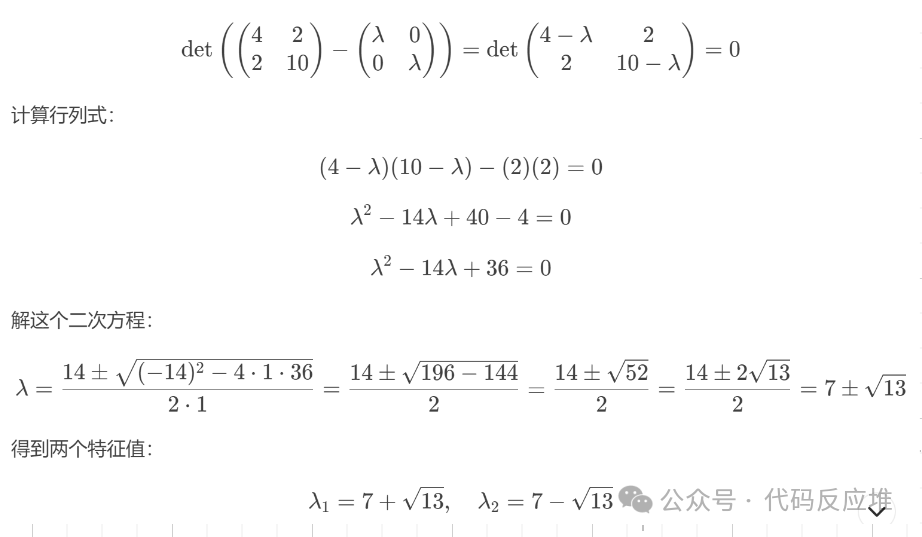
For an n × n square matrix, its characteristic equation det(A – λI) = 0 is an n-degree polynomial equation in λ (called the characteristic polynomial). According to the fundamental theorem of algebra, an n-degree polynomial equation has exactly n roots in the complex domain, thus an n × n matrix indeed has n eigenvalues.

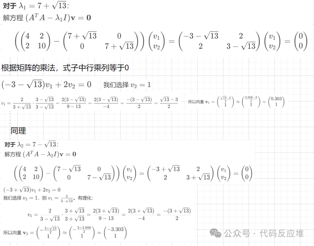
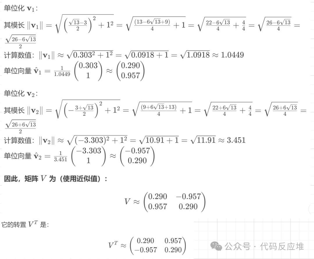
Then calculate the corresponding eigenvector and normalize it to ultimately obtain the basis unit matrix Vᵀ:

The matrix generated by multiplying itself after transposition is called a real symmetric matrix, and the eigenvectors corresponding to different eigenvalues are orthogonal to each other, meaning they are geometrically perpendicular. If these eigenvectors are normalized, they are called a set of standard orthogonal bases, and the matrix formed by directly using the standard orthogonal eigenvectors as columns is called an orthogonal matrix V. In AdaLoRA, the columns of this matrix V indicate the important “directions” in parameter updates.

The purpose of normalization is to convert the original eigenvectors into vectors of length 1. The length of 1 is derived using the Pythagorean theorem, where the modulus is calculated, and each number in the matrix is divided by the modulus, effectively proportionally reducing the values, with the ratio derived from calculations similar to the Pythagorean theorem.

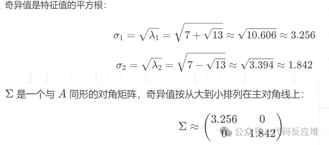
2. Calculating Σ (Singular Values)

Meaning: Scaling operation for each feature, representing the importance of each feature.

Constructing the singular value matrix Σ

3. Calculating U (Left Singular Vector)

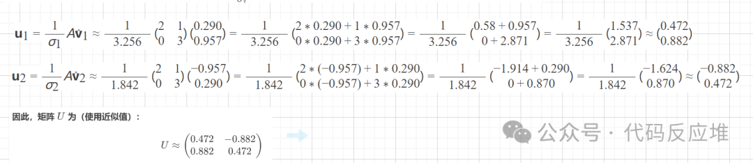
Meaning: A basic unit matrix on the minimum unit in the row space coordinate system (similarity between features), ensuring the results are presented correctly for use.

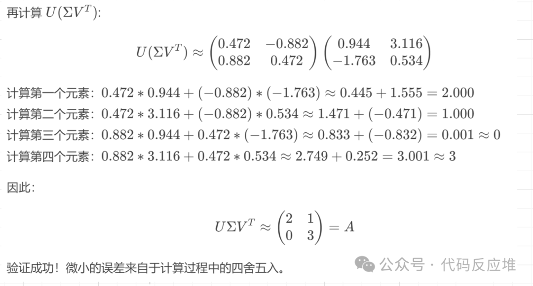
All intensities of different features recorded are multiplied together; if the values are closer, it indicates that these two records are very similar in their ratings for all movies. Similarly, the orthogonal matrix transposition Vᵀ is calculated, but there is a key mathematical conclusion that simplifies the calculation: the mathematical conclusion states that AAᵀ and AᵀA have exactly the same non-zero eigenvalues. Once the eigenvalues vᵢ and singular values σᵢ are known, the unit vector can be directly calculated using the following formula.

4. Final Results and Verification

A = U Σ Vᵀ

Issues with LoRA

Introduction to AdaLoRA

SVD Decomposition Instead of Low-Rank Matrices

1. Calculating Importance Scores

2. Substituting Importance Scores into SVD

Dynamic Pruning Fine-Tuning

1. Setting Goals

2. Initial Training (Initial Phase)

3. Model Pruning (Mid-Phase)

4. Stabilization Phase

5. Budget Scheduling for Each Phase

AdaLoRA Experimental Data

Introduction to SVD Derivation

0. Introduction

1. Calculating Vᵀ (Right Singular Vector) (Right Singular Vector)

2. Calculating Σ (Singular Values)

3. Calculating U (Left Singular Vector)

4. Final Results and Verification

Related posts

Leave a Comment Cancel reply