How to Build a High-Precision Rotary Transformer Simulator with Fault Injection Features?

Due to the ability of rotary transformers to maintain excellent reliability and high precision performance in harsh and adverse environments for a long time, they are widely used in applications such as EV, HEV, EPS, inverters, servos, railways, high-speed trains, and other applications that require obtaining position and speed information.

In the above system, many rotary transformer conversion chips (RDC), such as ADI’s AD2S1210 and AD2S1205, are used to obtain digital position and speed data.Customers’ systems often experience interference and failure issues, and many times they want to evaluate the accuracy performance of angle and speed under disturbed conditions, identify and verify the root causes of the problems, and then repair and optimize the system.A high-precision rotary transformer simulation system with fault injection capabilities (simulating the rotary transformer connected to a real motor running at a constant speed or fixed position) can address interference and fault issues without the need to build a complex motor control system.

This article will first analyze the error contributions in the rotary transformer simulation system and provide some error calculation examples to help you understand why high precision is so important for rotary transformer simulators. Then it will showcase fault examples under interference conditions in field applications. Next, it will introduce how to use the latest high-precision products to build a high-precision rotary transformer simulator with fault simulation and injection capabilities. Finally, it will demonstrate the functionalities that the rotary transformer simulator can achieve.

First, this section will introduce the ideal structure of a rotary transformer. Then, five common non-ideal characteristics and error analysis methods will be provided to help you understand why high precision is needed in rotary transformer simulator systems.

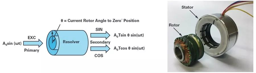
Figure 1. Structure of a rotary transformer.

As shown in Figure 1, the rotary transformer simulator simulates the connection to a rotary transformer of a real motor running at a constant speed or fixed position. Classical or variable reluctance rotary transformers consist of a rotor and a stator. A rotary transformer can be viewed as a special type of transformer. On the primary side, as shown in Equation 1, EXC represents the sine excitation input signal. On the secondary side, as shown in Equations 2 and 3, SIN and COS represent the modulated sine and cosine signals at the two output terminals.

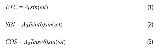
Where:

θ is the shaft angle, ω is the excitation signal frequency, A0 is the excitation signal amplitude, T is the rotary transformer transformation ratio.

The modulated SIN/COS signals are shown in Figure 2. For a constant angle θ in different quadrants, SIN/COS signals exhibit in-phase and out-of-phase conditions. For constant speed, the frequency of the SIN/COS envelope is constant, indicating speed information.

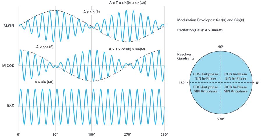
Figure 2. Electrical signals of the rotary transformer.

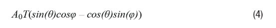
For all RDC products from ADI, the demodulated signal is represented as shown in Equation 4. When φ (output digital angle) equals the angle θ of the rotary transformer (position of the rotor), the Type II tracking loop is completed. In a real rotary transformer system, five non-ideal conditions may occur: amplitude mismatch, phase shift, incomplete orthogonality, harmonic excitation, and induced harmonics, leading to errors.

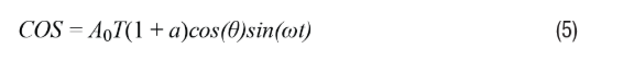
Amplitude mismatch is the difference in peak-to-peak amplitude when the SIN and COS signals reach their peak amplitude (COS at 0° and 180°, SIN at 90° and 270°). Differences in the winding of the rotary transformer or unbalanced gain control of the SIN/COS signals may lead to mismatch. To determine the position error caused by amplitude mismatch, Equation 3 can be modified to Equation 5.

Where a represents the amount of mismatch between the SIN and COS signals, and the remaining envelope signal after demodulation can be easily displayed as shown in Equation 6. By setting Equation 6 to equal to 0 to force the envelope signal in the Type II tracking loop to zero, we can find the position error ε=θ–φ. We can then obtain the error information, as shown in Equation 7.

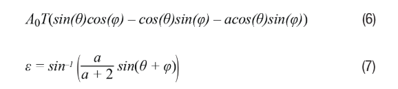
In real situations, if a is small, the position error is also small, meaning sin(ε)≈ε and θ+φ≈2θ. Therefore, Equation 7 becomes Equation 8, with the error term expressed in radians.

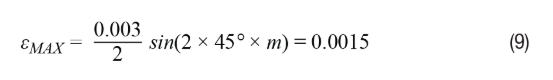
As shown in Equation 8, the error term fluctuates at twice the rotational speed, with the maximum error a/2 occurring at odd multiples of 45°. Assuming the amplitude mismatch is 0.3%, substituting the variables in Equation 8 and using odd multiples of 45°, the maximum error will be represented in Equation 9, where m is an odd integer.

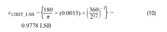
When the RDC mode is 12 bits, the error calculated in radians can be converted to LSB using Equation 10, approximately equal to 1 LSB.

Phase shift includes differential mode phase shift and common mode phase shift.Differential mode phase shift is the phase shift between the SIN and COS signals of the rotary transformer.Common mode phase shift is the phase shift between the excitation reference signal and the SIN and COS signals.To determine the position error caused by differential mode phase shift, Equation 3 can be modified to Equation 11.

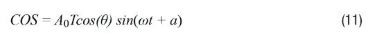
Where a represents the differential mode phase shift, and when the orthogonal term cos(wt)(sin(a)sin(θ)cos(φ)) is neglected, the remaining envelope signal after demodulation can be represented using Equation 12. In real situations, when a is small, cos(a)≈1–a²/2. By setting Equation 10 to equal to 0 to force the envelope signal in the Type II tracking loop to zero, we can find the resulting position error ε=θ–φ. We can then obtain the error information, as shown in Equation 13.

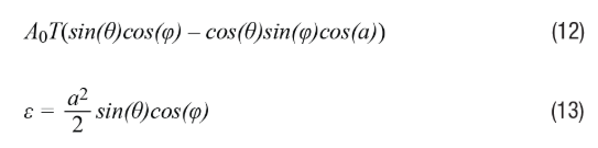
When θ≈φ, at θ≈45°, the maximum value of sin(θ)cos(φ) is 0.5. Therefore, Equation 13 becomes Equation 14, with the error term expressed in radians.

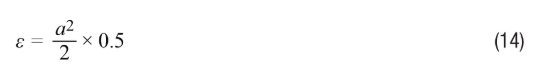
Assuming the differential mode phase shift is 4.44°, when the RDC mode is 12 bits, the error value can be converted to LSB using Equation 15, approximately equal to 1 LSB.

When the common mode phase shift is β, Equations 2 and 3 can be rewritten as Equations 16 and 17, respectively.

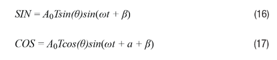
Similarly, the error term can be expressed using Equation 18.

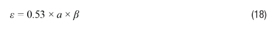
Under static working conditions, common mode phase shift does not affect the accuracy of the converter, but due to rotor impedance and the reactive component of the target signal, a moving rotary transformer will generate speed voltage. The speed voltage lies within the quadrant of the target signal and only occurs during motion; it does not exist at static angles. When the common mode phase shift is β, the tracking error can almost be represented using Equation 19, where ωM is the motor speed and ωE is the excitation speed.

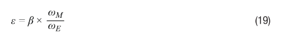
As shown in Equation 19, the error is proportional to the speed of the rotary transformer and the phase shift. Therefore, in general, using a high excitation frequency for the rotary transformer is beneficial.

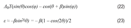
Incomplete orthogonality indicates that the two rotary transformer signals referred to by SIN/COS are not accurately 90° orthogonal. This occurs when the two rotary transformers are not processed or assembled in a completely spatially orthogonal manner. When β represents the amount of incomplete orthogonality, Equations 2 and 3 can be rewritten as Equations 20 and 21, respectively.

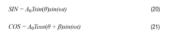
As before, the remaining envelope signal after demodulation can be easily displayed as shown in Equation 22. When you set the value of Equation 22 to 0, assuming β is small, cos(β)≈1 and sin(β)≈β, you can find the resulting position error ε=θ–φ. We can then receive the error information, as shown in Equation 23.

As shown in Equation 23, when the maximum error of β/2 reaches odd multiples of 45°, the error term fluctuates at twice the rotational speed. Compared to the error caused by amplitude mismatch, in this case, the average error is non-zero, and the peak error is equal to the orthogonal error. In the amplitude mismatch example, when β=0.0003 and radians=0.172°, approximately 1 LBS of error may occur in 12-bit mode.

In the previous analysis, it was assumed that the excitation signal is an ideal sine wave without additional harmonics. In actual systems, the excitation signal indeed contains harmonics. Therefore, Equations 2 and 3 can be rewritten as Equations 24 and 25, respectively.

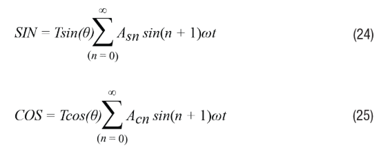
The remaining envelope signal after demodulation can be easily displayed as shown in Equation 26. In the Type II tracking loop, this signal is forced to zero.

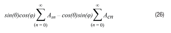
Setting Equation 26 to 0, we can find the resulting position error ε=θ–φ. We can then obtain the error information, as shown in Equation 27.

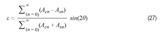
If the rotary transformer excitation contains the same harmonics, the numerator of Equation 27 is zero, resulting in no position error. This means that even when the values are very large, the effect of common excitation harmonics on the RDC can be negligible. However, if the harmonic content in SIN or COS differs, the resulting position error has the same functional shape as the amplitude mismatch shown in Equation 8. This can severely affect position accuracy.

In practice, it is impossible to establish an inductive curve that is a perfect sine and cosine function of position for a rotary transformer. Normally, harmonics are included in the inductance, and the VR rotary transformer contains a DC component. Therefore, Equations 2 and 3 can be rewritten as Equations 28 and 29, respectively, where K0 represents the DC component.

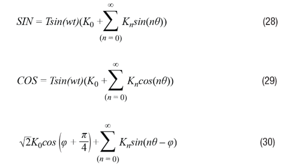
The remaining envelope signal after demodulation can be represented as shown in Equation 30.

In the Type II tracking loop, forcing this signal to zero, when the harmonic amplitude is small, n>1, and Kn<<1, the error information ε=θ–φ can be calculated using Equation 31.

According to this equation, compared to harmonic effects, the error is more sensitive to DC terms, and it is proportional to the amplitude of the induced harmonics. Meanwhile, the nth inductive harmonic determines the amplitude of the (n – 1)th harmonic of the position error.

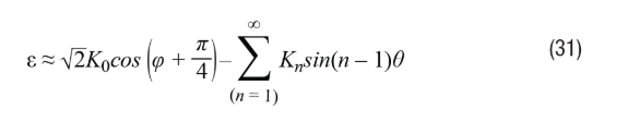
In addition to the error sources mentioned above, interference coupled to the SIN and COS lines, amplifier offset errors, bias errors, etc., can also lead to system errors. The summary of error sources and contributions in the rotary transformer simulator system is shown in Table 1, which includes the worst-case example of 1 LSB in 12-bit mode. This table can also be referenced to calculate the values for another RDC resolution mode.

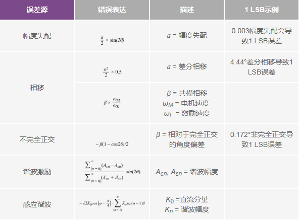
Table 1. Summary of Error Sources and Contributions in Rotary Transformer Simulator Systems

In real RDC systems, a large number of fault situations can occur. The following sections will show different types of faults that occurred during field testing and some fault signals, as well as how to use the rotary transformer simulator solutions introduced in Section 3 to simulate fault types. In addition to the aforementioned fault types, there may also be random interference leading to another fault, or some other faults occurring simultaneously.

Misconnection refers to incorrectly connecting the rotary transformer excitation and SIN/COS to the RDC SIN/COS input and excitation output pins. When misconnection occurs, the RDC can also decode angle and speed information, but the angle output data will show jumps, similar to a bias error in DAC output. Please refer to Figure 3 for the misconnection case and result data. The first column shows the EXC/SIN/COS pins and output angle, while the remaining columns show the misconnection situation.

Figure 3. Misconnection of the rotary transformer and angle output.

From the error contribution section, we learned that phase shift includes differential mode phase shift and common mode phase shift.Given that differential mode phase can be viewed as the difference of common mode phase shift, in this section, phase shift fault refers to faults caused by common mode phase shift.

Please refer to Figure 4 to see the contribution of common mode phase shift error. Phase 1 represents the delay of the excitation filter. Phase 2 represents the phase shift of the rotary transformer. Phase 3 represents line delay. Phase 4 represents the delay of the SIN/COS filter. In the field RDC system, when phase shift errors occur, it means that the total value of phase 1, phase 2, phase 3, and phase 4 exceeds 44°. Normally, the phase shift error of the rotary transformer is 10°. Under abnormal circumstances, the total phase error can reach 30°. Sufficient phase margin needs to be left for mass production considerations.

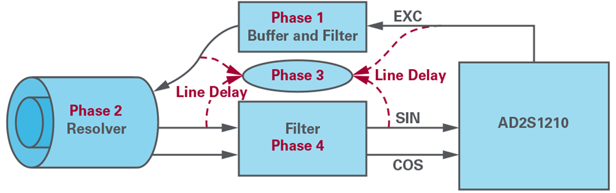
Figure 4. Contribution of phase shift error.

A disconnection fault occurs when any line of the rotary transformer is disconnected from the RDC platform interface. As product safety levels continuously improve, line disconnection detection has repeatedly attracted customer attention. We can simulate this fault by setting the SIN/COS to zero voltage. When a disconnection occurs, the LOS/DOS/LOT fault can be triggered in AD2S1210.

Amplitude mismatch occurs when the circuit gain control or the ratio of the rotary transformer for SIN/COS differs, which also means that the amplitude values of the SIN/COS envelope are different. When the amplitude approaches AVDD, an amplitude overlimit fault will be triggered. For AD2S1210, this is known as a clipping fault. Please refer to Figure 5 for an example of a good SIN/COS signal.

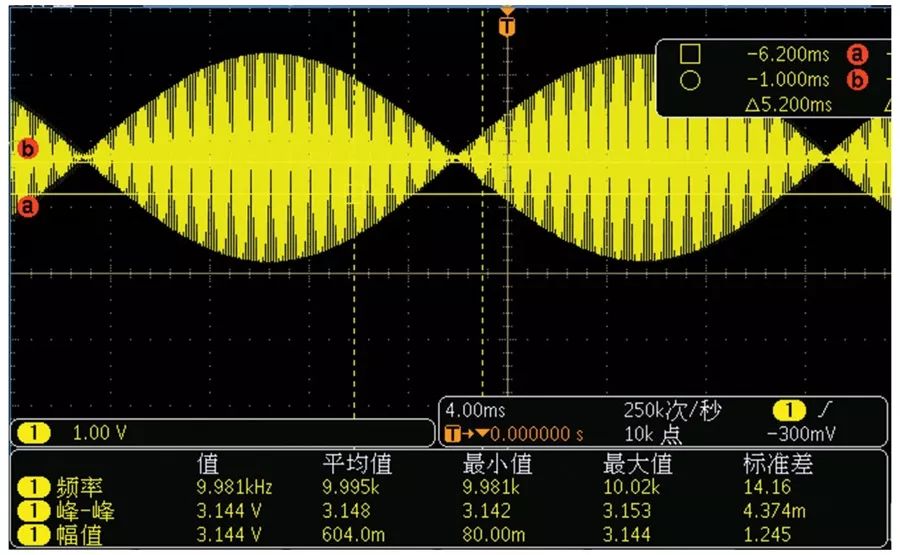
Figure 5. Ideal SIN/COS signal.

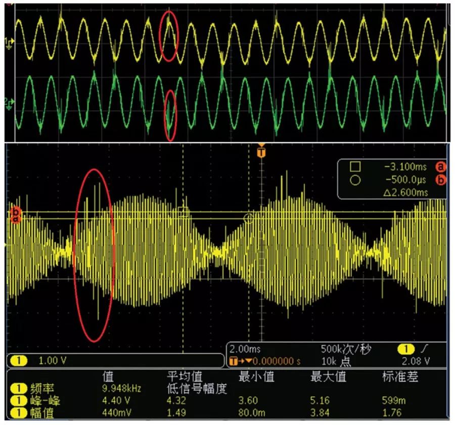
Figure 6. SIN/COS coupling IGBT interference.

IGBT interference refers to the coupling of interference signals with the on/off effects of IGBT switches. When signals couple with the SIN/COS lines, position and speed performance are affected, angle values may jump, and speed direction may change. Figure 6 shows a field example where channel 1 is the SIN signal, channel 2 is the COS signal, and the spikes indicate interference coupled with the IGBT switch.

An overspeed fault occurs when the speed of the electrical angle exceeds the speed of the rotary transformer decoding system. For example, in 12-bit mode, the maximum speed supported by AD2S1210 is 1250 SPS, and when the speed of the rotary transformer electrical angle is 1300 SPS, an overspeed fault will be triggered.

From the first section, we know that amplitude and phase errors will directly determine the decoding angle and speed performance. Fortunately, ADI provides a large precision product portfolio from which you can choose the right products to build a rotary transformer simulator system. The following description will demonstrate how to build a high-precision rotary transformer simulator and discuss which devices to select.

For the simulator block diagram shown in Figure 7, there are 7 modules to note:

1. Process control platform for data analysis and control.

2. Synchronous clock generation module to generate synchronous clocks for subsystems.

3. Fault signal generation module to generate different fault signals.

4. SIN/COS generation module to generate modulated SIN/COS signals as the output of the rotary transformer.

5. Signal acquisition module for collecting excitation and feedback signals.

6. SIN/COS output module that processes SIN/COS output containing buffers, gain, and filters.

7. Excitation signal input module with built-in buffering and filtering circuits.

8. Power module to provide power for ADC, DAC, switches, amplifiers, and other components.

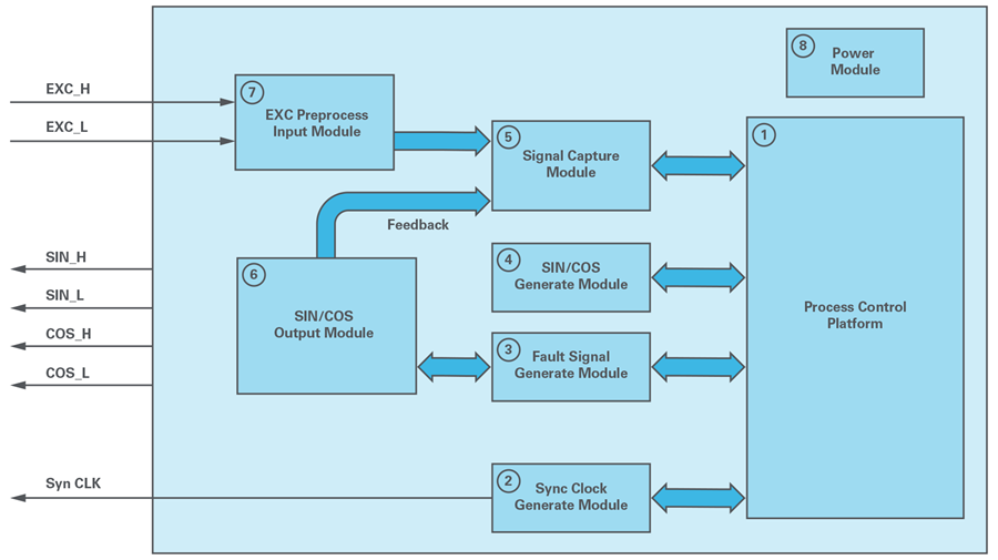
Figure 7. Rotary Transformer Simulator Block Diagram.

When the rotary transformer simulator system operates, the signal acquisition module collects excitation signal samples from the input module, which are then analyzed by the processor for their frequency and amplitude. The processor uses the CORDIC algorithm to compute the SIN/COS DAC output data code, and then generates a sine signal with the same frequency as the excitation input through the SIN/COS module. The system will simultaneously collect excitation and SIN/COS signals, calculate and adjust the SIN/COS phase/amplitude, compensating for the phase error between the excitation and SIN/COS to make it zero, and then calibrate the SIN/COS amplitude to the same level. Finally, the system generates modulated SIN/COS signals and fault signals to simulate angle performance, speed, and fault conditions.

Figure 8 shows the signal chain with a dual 16-bit sim SAR ADC AD7380 used for collecting excitation and feedback signals, achieving an SNR of up to 98 dB when OSR is enabled. It is very suitable for simultaneously collecting high-precision phase and amplitude calibration data. The ultra-low power, low distortion ADA4940-2 is used as the ADC driver. A high-precision, low-noise 20-bit DAC AD5791 is used to generate SIN/COS signals and fault signals, while for reducing resolution and cost, AD5541A or AD5781 can be used as substitutes for AD5791. A high-precision, selectable gain differential amplifier AD8475 is used as the input/output buffer. High-precision, ultra-low offset drift, and voltage noise amplifying operational amplifiers AD8676 and AD8599 are used to build active filters and summing circuits. A single-supply, rail-to-rail dual SPDT ADG854 with a maximum resistance of 0.8 Ω is used to switch and select SIN/COS signals, which are then sent to the data acquisition module.

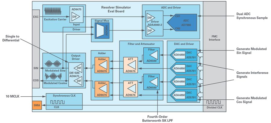
Figure 8. Signal Chain of the Rotary Transformer Simulator.

The entire rotary transformer simulator system is powered by an external 12V adapter, which uses a DC-DC converter and LDO voltage regulator to provide different voltage levels. Refer to Figure 9 for a detailed power signal chain. Using ADP5071, positive and negative 16V voltages can be generated, while using ADP7118 and ADP7182, clearer and more stable positive and negative 15V voltages can be generated. These power supplies are mainly used to power DAC-related circuits. Similarly, ADP2300, ADP7118, ADM660, and AD7182 can be used. These power supplies are primarily used to power ADC-related circuits and meet detailed design requirements.

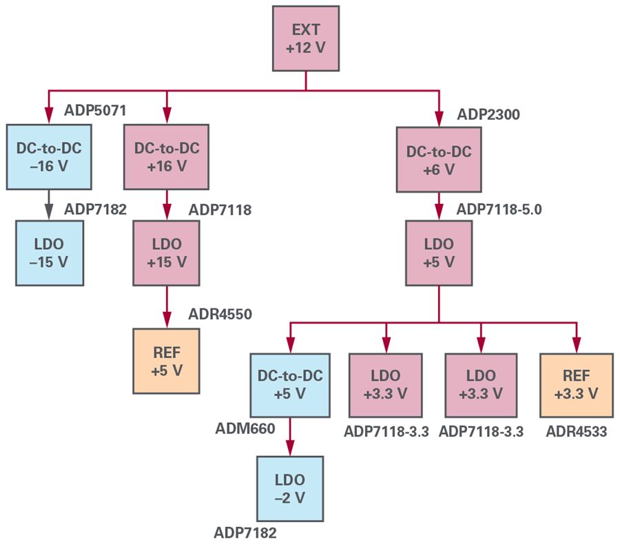
Figure 9. Power Signal Chain.

Refer to Figure 10 for the complete system platform testing. It includes a rotary transformer simulator board, an AD2S1210 evaluation board, and a GUI. See Figure 11 for the GUI and platform testing diagram. The AD2S1210 GUI is used to directly evaluate the performance of the rotary transformer simulator, especially angle and speed performance. The rotary transformer simulator GUI allows you to configure speed, angle performance, and fault signals.

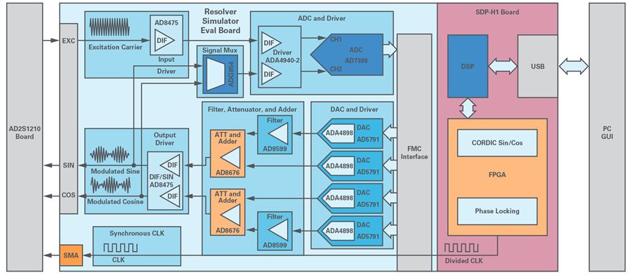
Figure 10. Experimental Testing Block Diagram.

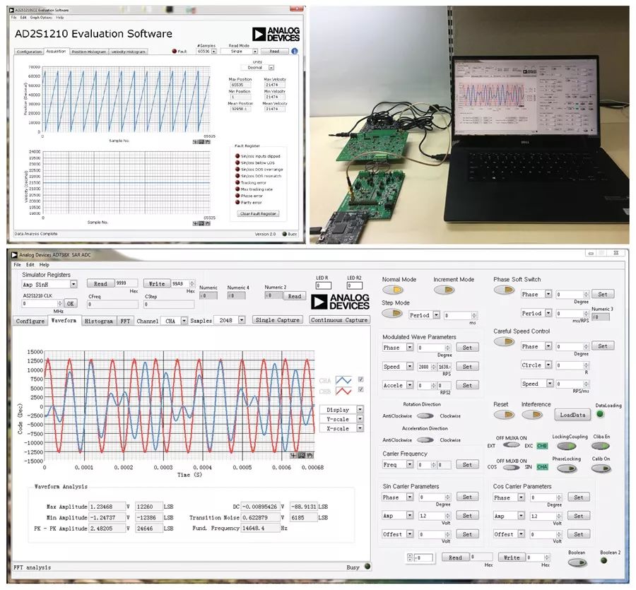
Figure 11. Experimental Testing and GUI.

Refer to Figure 12 for the angle and speed performance INL of the 16-bit AD2S1210 with the hysteresis mode disabled.

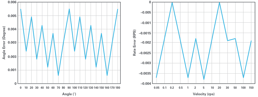
Figure 12. Angle/Speed INL.

Please refer to Table 2 for the performance data of this solution compared to standard rotary transformer simulator devices. The theoretical angle accuracy derived using AD5791 is 0.0004°, with an actual benchmark angle accuracy of 0.006°, and a maximum speed output of 3000 rps with a speed accuracy of 0.004 rps, easily meeting the requirements of AD2S1210 in 10 to about 16-bit modes.

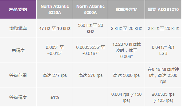
Table 2. Performance Comparison

Refer to Table 3 for the fault modes supported by this simulator. For phase-related faults, a range from 0° to about 360° can support SIN/COS signals. For amplitude-related faults, a range from 0 V to about 5 V can support SIN/COS signals. This solution can also be used to simulate overspeed, IGBT, disconnection, and other faults.

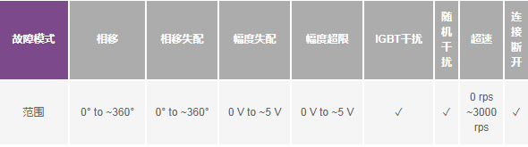
Table 3. Fault Modes and Supported Ranges

Refer to Figure 13 for a test example regarding IGBT faults. The simulator output is configured to 45°, and then a periodic interference signal is added to the SIN/COS output. From the angle and speed performance displayed on the AD2S1210 evaluation board GUI, it can be seen that the angle performance fluctuates around 45°, while the speed fluctuates around 0 rps.

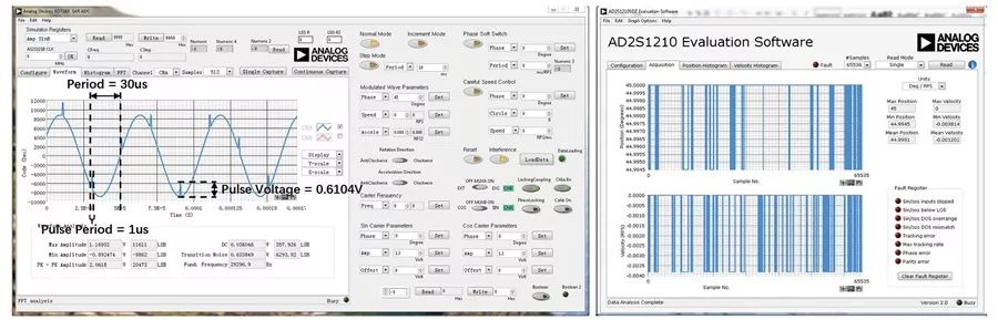
Figure 13. IGBT Interference Example.