Bluetooth’s wideband voice calls differ from narrowband voice primarily in the sampling rate, which increases from 8k to 16k, and the codec changes from CVSD to mSBC (modified SBC). The HFP (Hands-Free Profile) related to Bluetooth voice calls strongly recommends using a packet loss concealment (PLC) algorithm during wideband voice calls to ensure voice quality during packet loss, and provides a recommended floating-point implementation of the PLC algorithm. Since this is done on an ADSP with limited computing power, the floating-point implementation cannot be used directly, so it needs to be converted to fixed-point. Below, I will explain how I performed this conversion.
1. Understanding the Floating-Point Implementation of the Algorithm
The algorithm implementation is based on the paper “Waveform Substitution Techniques for Recovering Missing Speech Segments in Packet Voice Communications.” There are not many functions; the main APIs include three: InitPLC() for initialization, PLC_good_frame() for normal frame processing, and PLC_bad_frame() for processing lost frames. There are also three internal functions: CrossCorrelation() for calculating cross-correlation, PatternMatch() for determining the starting position of the best match, and AmplitudeMatch() for calculating the scale factor based on the best match position. These functions are called when processing lost frames.
2. Creating a Packet Loss Concealment Demo Combined with mSBC Implementation
Previously, there was only an SBC codec demo for Bluetooth music playback (based on BlueZ). To support mSBC, modifications were made to the SBC code (the core algorithm remains unchanged, but peripheral code was modified to support mSBC). Now, to combine PLC for packet loss concealment, the PLC code needs to be embedded into the mSBC decoding program. The general steps for creating the packet loss concealment demo are as follows:
1) Encode a segment of 16k sampled voice PCM into an SBC bitstream using the mSBC encoding program.
2) Decode the SBC bitstream back into PCM using the mSBC decoding program.
3) Embed the PLC code into the mSBC decoding program. Assuming one frame is lost every 100 frames (i.e., a packet loss rate of 1%), use the PLC algorithm to compensate for the lost frame and observe the compensation effect. The compensated voice should sound normal. This PLC algorithm and implementation are recommended in HFP and theoretically should not have issues. If the sound is abnormal after compensation, it is generally due to improper use of the API.
3. Fixed-Point Implementation of the PLC Algorithm
Before performing fixed-point implementation, it is necessary to identify the points that need conversion. By reviewing the code, I found three areas that require fixed-point conversion. Let’s look at how these three areas are converted to fixed-point.
1) Fixed-Point Conversion of the Cosine Table
There is a floating-point cosine table in the code, as shown below:

It needs to be converted into a fixed-point table. Looking at the range of values in the table, the absolute values are all less than 1, so it is suitable to use Q0.15 for fixed-point representation. Thus, the floating-point table is converted into a fixed-point table, as shown below:
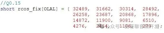
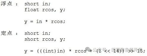
In the code, when using the cosine table, it is multiplied by PCM values. Since both are short values, care must be taken to avoid overflow, so one value must be explicitly cast to int before multiplication. After multiplication, a shift operation (right shift by 15 bits) is performed. To make the value closer to the floating-point value before shifting, rounding (adding 1<<14, i.e., adding 0.5) is applied. The example code is as follows:
2) Fixed-Point Implementation of Cross-Correlation Calculation
The code for calculating cross-correlation is as follows:
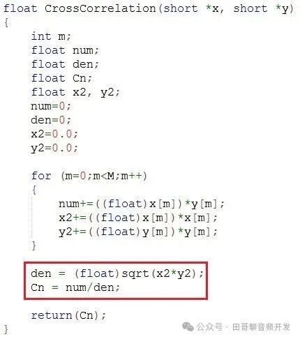
From the code, the formula used is as follows:
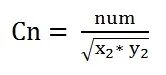
This involves both square root calculation and division. Previously, during code optimization, I learned that square roots can be calculated using Newton’s iteration method, so I looked for existing code in the AMR-WB reference code (mainly related to basic operations). Not only did I find it, but it also calculates the reciprocal of the square root (Word32 Isqrt(Word32 L_x), where the input is a 32-bit value and the output is a Q0.31 value), thus transforming division into multiplication. I tested the function Isqrt() with several values (e.g., 100), and the Q0.31 result matched the floating-point value. The formula then becomes:
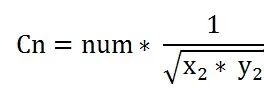
In the code, x2 and y2 are both 32-bit values, and their multiplication may exceed 32 bits. Since Isqrt() takes a 32-bit input, it cannot be used directly; some transformation is needed to convert it into the form m * 22n (where m is a 16-bit integer and n is a positive integer).

At this point, m1 * m2 is a number within 32 bits, allowing the use of the function Isqrt().

 Using Isqrt(),
  is simply right-shifting (n1 + n2) bits. The result is then multiplied by num to obtain the fixed-point Cn.
3) Fixed-Point Implementation of Division
In the floating-point implementation, division is used when calculating the scale factor, as shown in the code below:
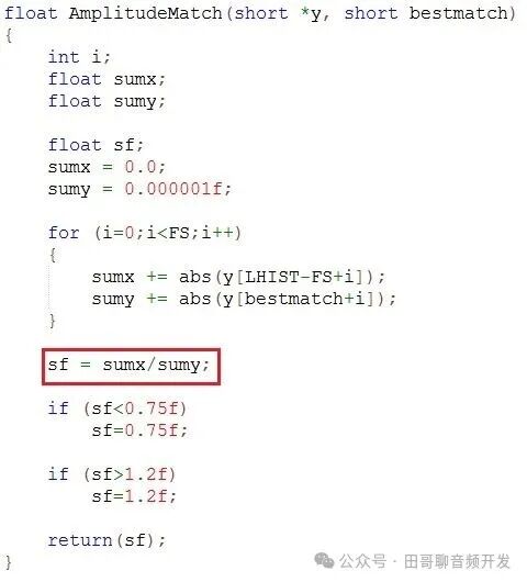
Looking at the AMR-WB reference code, there is also a division implementation, namely Word16 div_s (Word16 var1, Word16 var2). However, this is a 16-bit division, and the output is also a Q0.15 16-bit value. There are additional constraints when using it: both the dividend and divisor must be positive, and the dividend must be less than or equal to the divisor. In the floating-point code, both the dividend and divisor can be 32-bit positive values, so direct use is not possible; some modifications are needed to convert it into the form m * 2n (where m is a positive integer within 16 bits and n is a positive integer).

Using div_s() to calculate m1/m2, 2(n1-n2) represents the shift (left shift, right shift, or no shift). From the floating-point code, the scale factor ranges from 0.75 to 1.2, which should be represented in Q1.14 format. Therefore, the Q0.15 value obtained from div_s() needs to be converted to Q1.14 format. Finally, a clamping is applied, with a range of 0.75 to 1.2, which in Q1.14 format corresponds to 12288 to 19661. After these processes, the fixed-point scale factor can be obtained.
During the fixed-point conversion process, each step’s fixed-point result must be compared with the floating-point result to ensure the error is within a very small range, typically not exceeding 1. After completion, the final error of the PCM values must also be compared. The following figure shows the comparison of the final PCM values between the floating-point and fixed-point implementations:
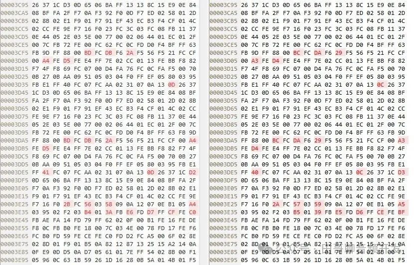
From the figure, it can be seen that during packet loss concealment, there are errors in the PCM values between the fixed-point and floating-point implementations, but the errors are all within the range of 1, which is acceptable.
To facilitate better communication and mutual assistance, I have created a discussion group. If you are interested, please scan the QR code below, and I will add you to the group. Thank you! AuthorIntroduction:
Master’s degree from a well-known 985 engineering university. Engaged in audio software development for nearly 20 years, previously employed by two Fortune 500 companies (one in chip design and the other in communication equipment), currently working at a chip design company listed on the Science and Technology Innovation Board. I have experience in many aspects of audio software development, and the articles I write are based on my work experiences and summaries. My technical blog has nearly 3000 followers. I hope you can find the valuable content you need here.