Kerckhoffs principle states that the security of a cryptographic system relies solely on the security of the key, with everything else in the system considered public information. However, in reality, software reverse engineering and dynamic/static debugging techniques have successfully executed key extraction attacks on cryptographic systems.
Given this fact, both the industry and academia have begun research on white-box cryptography. The goal of white-box cryptography is clear: to ensure the security of the key in a white-box attack environment. The successful application of differential computation analysis and differential fault analysis on white-box cryptography has brought new challenges to the field. This article primarily explains differential fault analysis and introduces an example of using the Unicorn framework for dynamic fault injection in white-box cryptography.


1. Principles


Due to space limitations, this section will not elaborate on the relevant theoretical knowledge but will provide supplementary information necessary for understanding the article. Readers can supplement their knowledge through the following links.
-
White-box Cryptography:A Tutorial on White-box AES
-
Differential Fault Analysis:DFA on Whitebox AES
1.1 White-box Block Ciphers
White-box cryptography is primarily designed around two modes:
-
Implementing a white-box version of an existing block cipher algorithm, such as the white-box implementations of AES and SM4.
-
Designing new white-box algorithms that can resist key extraction attacks, such as SPNBOX.
For the first mode, algorithm designers often convert key steps of the block cipher algorithm’s sbox into lookup table operations. Then, they encode and protect the lookup table. To ensure compatibility, designers typically do not apply encoding protection to the algorithm’s inputs and outputs. This directly leads to the fact that attack methods effective against standard block cipher algorithms can also be applied to the white-box implementations of these algorithms, such as differential fault analysis and differential computation analysis.
1.2 Differential Fault Analysis
1.2.1 Principles of Differential Fault Analysis
Differential Fault Analysis (DFA) can be understood as injecting faults at specified locations during the normal operation of a cryptographic system, causing the system to produce incorrect ciphertext. By performing differential analysis on the erroneous ciphertext and the correct ciphertext, and combining this with the input and output differential tables of the sbox, the round key can ultimately be obtained.
The overview of differential fault analysis is shown in the figure below:
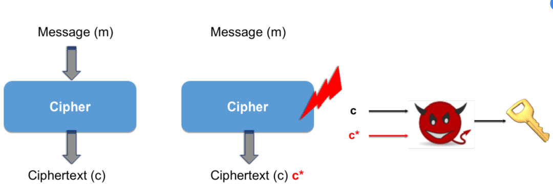
Assuming that the encryption program Cipher encrypts the message m, producing the ciphertext c after normal execution. An attacker captures both m and c and attempts to execute Cipher again with the same input m, injecting a fault just before a certain round of execution, causing Cipher to output c*. By combining the input and output differential distribution tables of the sbox, the attacker can extract the round key and subsequently recover the master key.
To facilitate understanding, this article uses a simple 3-bit encryption algorithm E as an example. The S-box corresponding to E is also 3 bits, as shown in the following table:
| 0 | 1 | 2 | 3 | 4 | 5 | 6 | 7 |
|---|---|---|---|---|---|---|---|
| 6 | 2 | 4 | 7 | 1 | 0 | 3 | 5 |
Through the above S-box, a nonlinear transformation can be performed in the cryptographic algorithm, such as: Sbox(3) = 7. Assume the encryption algorithm E is represented as follows:
Now, there is an implementation of E, unknown to the attacker A, who performs differential fault analysis on E. The specific steps are as follows:
1. Execute the program E normally, setting inputs to 6 and 2, obtaining outputs of 0 and 2, respectively, as shown in the table below:
| M | K | C |
|---|---|---|
| 6 | – | 0 |
| 2 | – | 2 |
2. The attacker A injects a fault during the execution of E (in this case, modifying the input). As shown in the table below:
| M’ | K | C’ |
|---|---|---|
| 7 | – | 1 |
| 5 | – | 3 |
3. To further analyze, the attacker A constructs an input differential and output differential distribution table based on the S-box. For understanding the differential distribution table, this article provides a small example: Sbox(0) = 6; Sbox(3)=7. Therefore, the input differential is , and the output differential is , at this point, it can be said that when the input differential is 3, and the output differential is 1, the S-box potentially has inputs of 0 and 3. For the sake of convenience in this example, the S-box used is 3 bits, while for the AES algorithm, the S-box is 8 bits, resulting in a much larger differential distribution table. The differential distribution table for this example’s S-box is shown in the table below, where the vertical axis represents input differentials, and the horizontal axis represents output differentials.
| DI\DO | 1 | 2 | 3 | 4 | 5 | 6 | 7 |
|---|---|---|---|---|---|---|---|
| 1 | 4,5 | 2,3 | 0,1 | 6,7 | |||
| 2 | 2,4,6 | 1,3,5,7 | |||||
| 3 | 0,3 | 5,6 | 4,7 | 1,2 | |||
| 4 | 1,3,5,7 | 0,2,4,6 | |||||
| 5 | 2,7 | 1,4 | 3,6 | 0,5 | |||
| 6 | 0,2,4,6 | 1,3,5,7 | |||||
| 7 | 1,6 | 0,7 | 2,5 | 3,4 |
4. By combining the input and output differential tables, the differential relationships of M and M’, C and C’ can be established, resulting in the following table:
| M M’ | C C’ | input (lookup table) | K=input M |
|---|---|---|---|
| 6 ^ 7 = 1 | 0 ^ 1 = 1 | {4,5} | {2,3} |
| 2 ^ 5 = 7 | 2 ^ 3 = 1 | {1,6} | {3,4} |
5. The two sets of candidate key values obtained are intersected, ultimately determining the key to be 3.
1.2.2 AES Differential Fault Analysis Based on Single-byte Faults
AES differential fault analysis based on single-byte faults was proposed by Dusart et al. in 2003. In this scheme, the attacker does not need to know the exact location and value of the injected fault; by analyzing the correct ciphertext and the erroneous ciphertext generated after fault injection, the tenth round key can be analyzed. Detailed content can be referenced in the article DFA on Whitebox AES (https://blog.quarkslab.com/differential-fault-analysis-on-white-box-aes-implementations.html). For a Chinese explanation, you can refer to the paper A NoisyRounds Protected White-box AES Implementation and Its Differential Fault Analysis (http://www.jcr.cacrnet.org.cn/CN/abstract/abstract396.shtml).
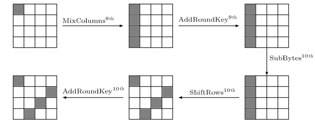
This scheme first injects a single-byte fault before the mix column operation in the 9th round, and after subsequent rounds of operations, it will produce ciphertext with faults, as shown in the figure below. These faulty ciphertexts and the correct ciphertext have a certain differential relationship, and by analyzing this differential relationship, the relationship between the S-box’s input and output differentials can be obtained, further determining the key.


2. Tools


2.1 Unicorn
Unicorn is a lightweight, multi-architecture CPU emulator. Due to its significant features, it is used by many reverse engineering practitioners and binary enthusiasts. Unicorn can hook in various ways, including but not limited to instruction hooks, memory read/write hooks, and read/write exception hooks. For differential fault analysis, the most crucial prerequisite is obtaining erroneous ciphertext that meets certain conditions, which the Unicorn framework can satisfy by hooking the instructions that read memory during program execution and modifying their data to achieve fault injection. However, Unicorn only simulates CPU functionality; for general binary programs, there are also system call functions such as: scanf, printf, strcpy, etc., which require users to hook and implement manually, necessitating a certain level of assembly skill.
2.2 Rainbow
Rainbow (https://github.com/Ledger-Donjon/rainbow) is a DBI tool open-sourced by the security research team of Ledger, a manufacturer of Bitcoin hardware wallets. This tool is developed based on Unicorn and encapsulates many practical features, significantly improving loading ELF files, reading/writing memory, and hooking functions. More importantly, this project is optimized for side-channel attacks, capable of automatically generating traces, which is particularly useful for differential computation analysis. This article will use this tool for DFA experiments.
2.3 PhoenixAES
PhoenixAES (https://github.com/SideChannelMarvels/JeanGrey/tree/master/phoenixAES) is a tool open-sourced by Side-Channel Marvels (a side-channel analysis research organization) for performing differential fault analysis on AES. Given sufficient erroneous ciphertext, this tool can analyze the round keys. After using the rainbow tool to obtain enough erroneous ciphertext, this article will use this tool for differential analysis to extract the round keys.


3. Implementation


3.1 Fault Injection
Fault injection in white-box block ciphers can be categorized into dynamic and static injection, which are introduced below:
Dynamic Injection: During the execution of the encryption program, faults can be injected by modifying register values, instructions, or values in memory. The advantage of this method is that faults can be injected anywhere during program execution. However, it requires users to have a certain level of reverse engineering and assembly knowledge.
Static Injection: Before the execution of the encryption program, faults can be injected by modifying the binary files that the program depends on. For example, a white-box encryption program often relies on a white-box lookup table, which may exist independently or be embedded within the encryption program. If faults are injected into this lookup table before executing the program and the program’s output changes, then the injection is successful. The advantage of this method is its simplicity; however, the drawbacks are also apparent. Firstly, there are many values in the white-box lookup table that will not be used, meaning injection may likely fail. Secondly, static injection cannot fully cover the details of the algorithm’s execution process. If the lookup table has certain protections, injection may also fail.
This article will use the rainbow tool to implement dynamic injection for the AES white-box algorithm whitebox. This example is from the RHME3 CTF.
3.1.1 Determining the Injection Interval
To inject faults more precisely before the mix column operation in the 9th round of the AES algorithm, the execution process of the white-box needs to be analyzed first, using the Tracer tool to record the execution process of the white-box. This tool is based on Ubuntu 18.04, and to facilitate usage, this article has pre-integrated the environment into a Docker image for convenience.
docker pull tobyssd/side_channel_tool_for_whitebox_cipher:latest
After entering the container, place the white-box file and execute the following command at the location of the white-box:
echo -n 00000000000000000000000000000000|Tracer -t sqlite -o rhme3.sqlite -- ./whitebox --stdinThis generates a trace record rhme3.sqlite, which is an SQLite database file that can be opened using Navicat or TraceGraph, which can be compiled and installed directly. The TraceGraph opens as shown in the figure below:
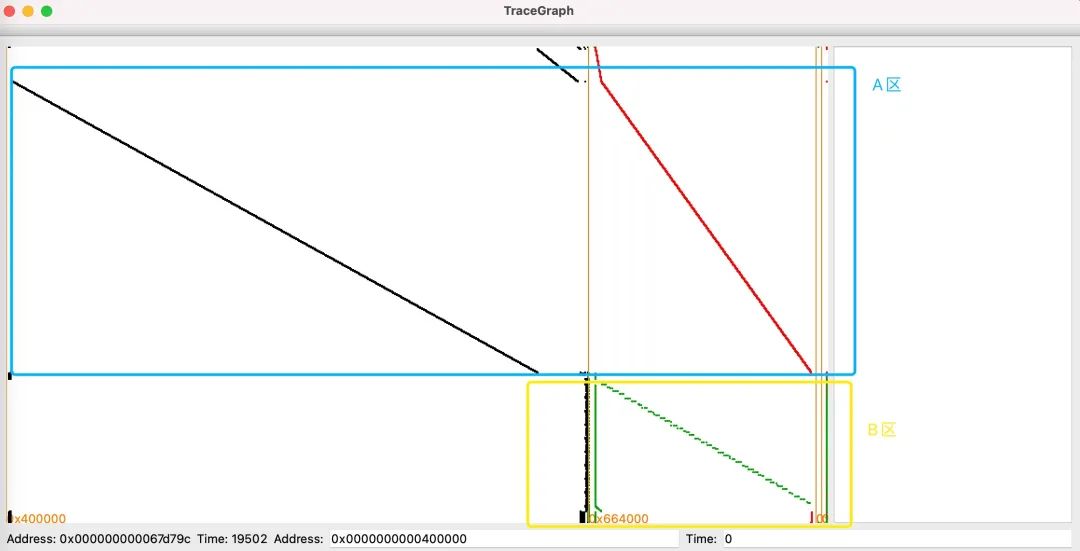
The vertical axis represents time, increasing from top to bottom. The horizontal axis represents addresses, increasing from left to right. Black indicates instruction execution, green indicates memory reads, red indicates memory writes, and orange indicates memory reads or writes. By using the zoom-in and zoom-out functions, the execution details can be made more detailed. In the area marked A, it can be seen that as time progresses, there are almost no repeated instructions, and corresponding to that, there are almost only write memory operations. Therefore, it is temporarily believed that this is the processing of the white-box table. In area B, as time progresses, the instruction set is concentrated on a small block of addresses, indicating that there are loop operations. We know that the AES algorithm has 10 rounds, so it is reasonable to have loop operations for 9 rounds. We define the injection range between the 8th and 9th rounds and find the corresponding memory interval, as shown in the figure, from 0x682000 to 0x689000.
3.1.2 Injecting Faults
After determining the injection interval, we can attempt to inject faults. Next, I will explain some details of the injection script.
-
Initializing the Environment
from rainbow.generics import rainbow_x64 # Import the rainbow environment e = rainbow_x64() # Generate a 64-bit virtual machine e.load("whitebox", typ=".elf") # Import the white-box program -
Hooking system call functions and implementing them manually
def pyprints(emu): src = emu['rdi'] i = 0 c = emu[src] while c != b'\x00': i += 1 c = emu[src+i] return True def pyput(emu): src = emu['rdi'] i = 0 c = emu[src] while c != b'\x00': i += 1 c = emu[src + i] return True def pystrlen(emu): src = emu['rdi'] i = 0 c = emu[src] while c != b'\x00': i += 1 c = emu[src + i] emu['rax'] = i return True def pystrncmp(emu): a = emu['rdi'] b = emu['rsi'] n = emu['rdx'] i = 0 flag = 0 for i in range(n): ar = emu[a+i] br = emu[b+i] if ar != br: flag = 1 break if flag == 0: emu['rax'] = 0 else: emu['rax'] = 1 return True def pystrncpy(emu): dest = emu['rdi'] src = emu['rsi'] n = emu['rdx'] for i in range(n): c = emu[src + i][0] emu[dest + i] = c return True e.stubbed_functions['puts'] = pyput e.stubbed_functions['strlen'] = pystrlen e.stubbed_functions['freopen'] = pystrlen e.stubbed_functions['strncmp'] = pystrncmp e.stubbed_functions['strncpy'] = pystrncpy e.stubbed_functions['printf'] = pyprints -
Manually setting the main function’s parameters (plaintext input)
input_buf = 0xCAFE1000 argv = 0xCAFE0000 e[input_buf] = b"0011223344556677" e[argv + 8] = input_buf e["rdi"] = 2 # argc e["rsi"] = argv -
Setting hooks,
# Mainly to determine if it has been injected and if the length is 4 bytes def should_fault(evtId, targetId, fault, address, size): return evtId > targetId and fault and size == 4 def hook_mem_access_fault(mu, access, address, size, value, user_data): global output, evtId, fault,p evtId += 1 targetId = user_data[0] if access == uc.UC_MEM_READ: # If it is a memory read operation, further judgment if should_fault(evtId, targetId, fault, address, size): print("FAULTING AT ", evtId) p = evtId fault = False bitfault = 1 << random.randint(0, 31) value = u32(mu.mem_read(address, size)) # Get the value to be read # Inject fault nv = p32(value ^ bitfault) e[address + 0] = nv[0] e[address + 1] = nv[1] e[address + 2] = nv[2] e[address + 3] = nv[3] # Where begin and end indicate the monitored memory interval e.emu.hook_add(uc.UC_HOOK_MEM_READ, hook_mem_access_fault, begin=0x682000,end=0x689000,user_data=target) -
Capturing ciphertext; after prior analysis, it was found that the ciphertext appears at instruction address 0x0400670, capturing rsi will yield the ciphertext.
def hook_code(mu, address, size, user_data):
    global output
# Obtain output
if address == 0x0400670:
    if e['rsi'] < 256:
        output.append(e['rsi'])

e.emu.hook_add(uc.UC_HOOK_CODE, hook_code)
The above analyzes some important details of the injection. For specific code, please refer to dfa_rhme3.
After successfully running the code, it takes about 5 minutes to obtain sufficient erroneous ciphertext.
3.2 Differential Fault Analysis
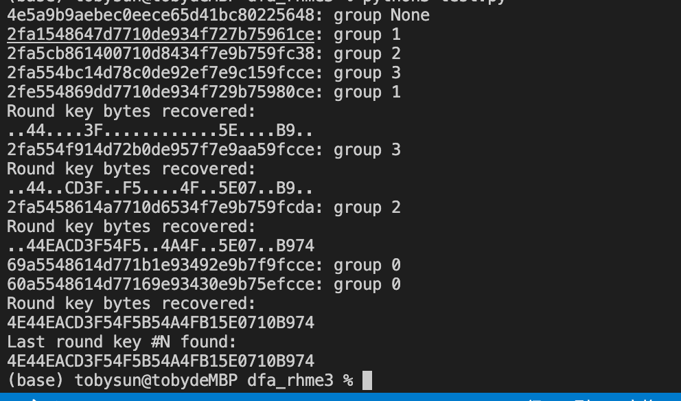
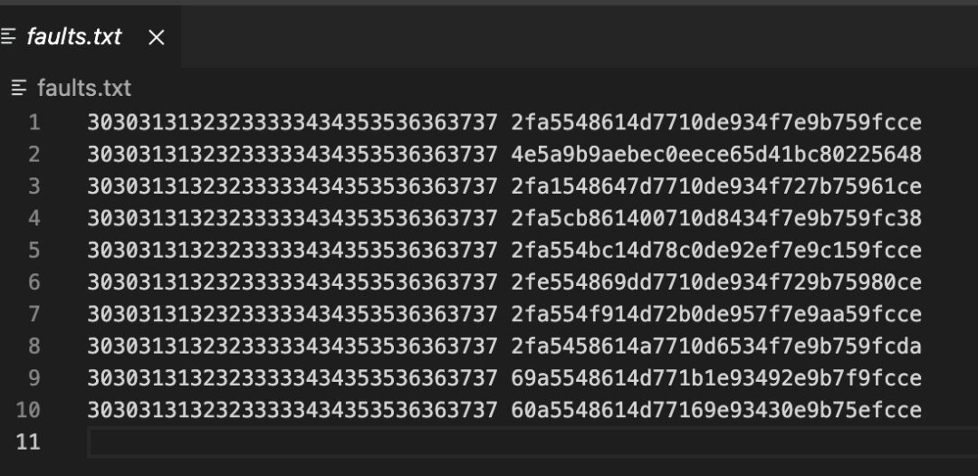
Using PhoenixAES to analyze the erroneous ciphertext will ultimately yield the round key.
import aes_dfa
aes_dfa.crack_file("faults.txt", verbose=2)
As shown, after obtaining the round key, based on the characteristics of AES key scheduling, it is possible to directly backtrack to the first round master key.