Hello, welcome to Crossin’s Programming Classroom!

For those engaged in scientific research, mathematical formulas are indispensable. However, displaying mathematical formulas in the program’s output can be quite challenging.

This article will introduce how to use LaTeX formulas and symbols in Matplotlib, as well as how Python can generate LaTeX mathematical formulas.

1. Using LaTeX formulas and symbols in Matplotlib

Some configurations

• Install two software packages, links provided.

• https://mirrors.cqu.edu.cn/CTAN/systems/windows/protext/protext-3.2-033020.zip
• https://github.com/ArtifexSoftware/ghostpdl-downloads/releases/download/gs9531/gs9531w64.exe

• Add to the environment variables

The following two lines should be added to the environment variable: C:\Users\xx\AppData\Local\Programs\MiKTeX 2.9\miktex\bin\x64;C:\Program Files\gs\gs9.53.1\bin;

• Modify matplotlib.rcParams

import numpy as np
import matplotlib as mpl
import matplotlib.pyplot as plt

plt.style.use('fivethirtyeight')
mpl.rcParams['text.usetex'] = True # Default is false, set to TRUE here

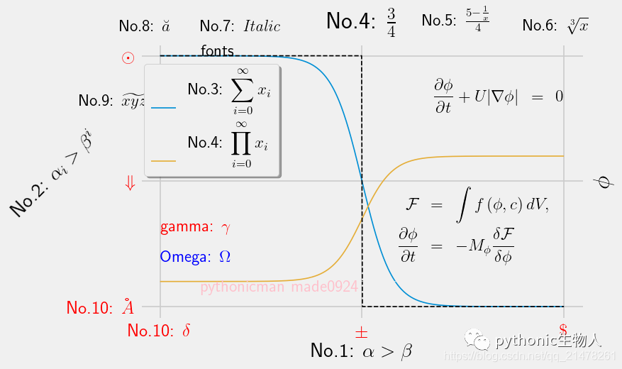
Using LaTeX characters and formulas in Matplotlib

mpl.rcParams['lines.linewidth'] = 1

fig, ax = plt.subplots(dpi=120)

N = 500
delta = 0.6
X = np.linspace(-1, 1, N)
ax.plot(X, (1 - np.tanh(4 * X / delta)) / 2,    
        X, (1.4 + np.tanh(4 * X / delta)) / 4, "C2", 
        X, X < 0, "k--")                        

ax.set_xlabel(r'No.1: $\alpha > \beta$')

# Superscripts and subscripts
ax.set_ylabel(r'No.2: $\alpha_i > \beta^i$, rotation=45)

# Accumulation
ax.legend((r'No.3: $\displaystyle\sum_{i=0}^\infty x_i$', r'No.4: $\displaystyle\prod_{i=0}^\infty x_i$),
          shadow=True, loc=(0.01, 0.52), handlelength=1.5)

# Fractions  
ax.set_title(r'No.4: $\frac{3}{4}$')

# Binomial
ax.text(0.3,1.1,r'No.5: $\frac{5 - \frac{1}{x}}{4}$')

# Square root
ax.text(0.8,1.1,r'No.6: $\sqrt[3]{x}$')

# Change font
## Roman, Italic, Typewriter, CALLIGRAPHY, etc.
ax.text(-0.8,1.1,r'No.7: $\mathit{Italic}$')
ax.text(-0.8,1.0,r'$\mathsf{fonts}$')

# Tone
ax.text(-1.2,1.1,r'No.8: $\breve a$')

# Select a range
ax.text(-1.4,0.8,r'No.9: $\widetilde{xyz}$')

# The arrow
ax.annotate("", xy=(-delta / 2., 0.1), xytext=(delta / 2., 0.1),
            arrowprops=dict(arrowstyle="<->", connectionstyle="arc3"))

# Other TeX symbols
ax.set_xticks([-1, 0, 1])
ax.set_xticklabels([r"No.10: $\delta$", r"$\pm$", r"$\$"], color="r", size=15)

ax.set_yticks([0, 0.5, 1])
ax.set_yticklabels([r"No.10: $\AA$", r"$\Downarrow$", "$\\odot$"], color="r", size=15)

ax.text(1.02, 0.5, r"$\phi$", fontsize=20, rotation=90,
        horizontalalignment="left", verticalalignment="center",
        clip_on=False, transform=ax.transAxes)

# Integral and differential formulas

# Equation 1
eq1 = (r"\begin{eqnarray*}"
       r"\frac{\partial \phi}{\partial t} + U|\nabla \phi| &=& 0 "
       r"\end{eqnarray*}")
ax.text(1, 0.9, eq1, horizontalalignment="right", verticalalignment="top")

# Equation 2
eq2 = (r"\begin{eqnarray*}"
       r"\mathcal{F} &=& \int f\left( \phi, c \right) dV, \\ "
       r"\frac{ \partial \phi } { \partial t } &=& -M_{ \phi } "
       r"\frac{ \delta \mathcal{F} } { \delta \phi }"
       r"\end{eqnarray*}")
ax.text(0.18, 0.18, eq2)

ax.text(-1, .30, r"gamma: $\gamma$", color="r")
ax.text(-1, .18, r"Omega: $\Omega$", color="b")

plt.show()

2. Using latexify to generate LaTeX mathematical formulas

import math
import latexify
@latexify.with_latex # Call the latexify decorator
def solve(a, b, c):
  return (-b + math.sqrt(b**2 - 4*a*c)) / (2*a)

solve

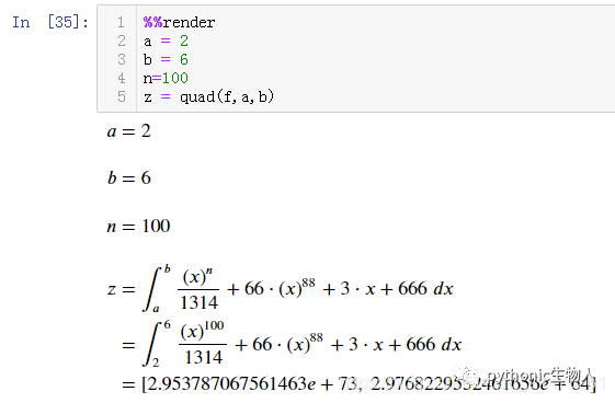
3. Using handcalcs to generate LaTeX mathematical formulas

• A formula for integration, using scipy’s quad

import handcalcs.render
from scipy.integrate import quad # Use scipy.quad for integration

%%render
a = 2
b = 6
n=100
z = quad(f,a,b)

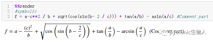
• A mixed formula, using the math module

from math import sqrt, cos, sin, tan, asin
import handcalcs.render

%%render
#symbolic
f = a - c**2 / b + sqrt(cos(sin(b - 2 / c))) + tan(a/b) - asin(a/c) #Comment part

4. LaTeX symbols reference table

Symbols were crawled from the website: https://matplotlib.org/tutorials/text/mathtext.html, a quick reference table was created.

plt.figure(dpi=400)
fig = sns.scatterplot(x='sepal length(cm)', y='sepal width(cm)', data=pd_iris,
            style=geek[:150], # Add different class variables according to different markers
            markers=[r"$" + geek[i] + "$" for i in range(150)], # Custom marker shapes
            **dict(s=320),
            color='#01a2d9'
           )

fig.legend(ncol=5,
           fontsize=10,
           loc=8,
           bbox_to_anchor=(0.45, 1), 
           facecolor='#eaeaea',
          )

sns.set(style="whitegrid", font_scale=1)

References

https://matplotlib.org/tutorials/text/usetex.html https://github.com/connorferster/handcalcs https://github.com/google/latexify_py

Thanks toeveryone who shared and liked this post~

Author: Pythonic Biologist

_Previous articles recommended_