Water vapor flux and water vapor flux divergence are important physical quantities in meteorology, playing a key role in the study of atmospheric water vapor transport, precipitation formation, and regional climate change. Water vapor flux reflects the amount of water vapor passing through a unit area per unit time, while water vapor flux divergence describes the convergence or diffusion of water vapor within a unit volume.
1
Representation and Integration Methods of Water Vapor Flux and Its Divergence(1) Water Vapor Flux FormulaIn the atmosphere, the three-dimensional water vapor flux vector F can be expressed as: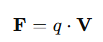 Where:
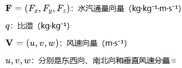 The commonly used vertical integral of water vapor flux (considering only horizontal components):
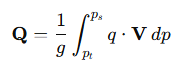 Where:
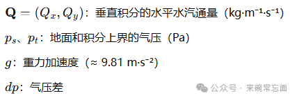 (2) Water Vapor Flux Divergence FormulaIn three-dimensional form:
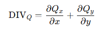
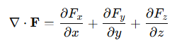 For the vertical integral of horizontal water vapor flux divergence:
 The vertical integral formula at p-coordinate is: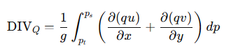
Water Vapor Flux: Represents the transport capacity and direction of water vapor in the entire atmospheric column, with the vector pointing in the direction of water vapor transport, and the magnitude proportional to the transport intensity.
Water Vapor Flux Divergence: Measures the net water vapor budget in a certain area.
Negative values (convergence): Favorable for precipitation occurrence.
Positive values (divergence): Favorable for drying.
In practical applications, the water vapor flux from 1000 hPa to 300 hPa is usually calculated to represent the total water vapor flux in the layer, which is applicable in most cases in most regions. However, in complex terrain areas, such as the typical Tibetan Plateau region, starting the integration from 1000 hPa poses problems because the average elevation of the Tibetan Plateau exceeds 4000 meters, roughly corresponding to 600 hPa. The portion below 600 hPa, including 1000 hPa, is underground, and due to the complex terrain in the plateau area, the calculated distribution of water vapor flux and its divergence appears very “strange” (figure omitted). Therefore, it is essential to calculate the water vapor flux and water vapor flux divergence from the surface to 300 hPa using surface pressure!
2
Issues and Solutions in Python ImplementationIn NCL, the thickness of pressure layers is usually calculated using the dpres_plevel_Wrap function, and then multiplied by the water vapor flux to obtain the vertical integral from the surface to 300 hPa. The author found that the water vapor flux divergence calculated using Python based on the same logic performed poorly in the southern Tibetan Plateau and some complex terrain areas of South Asia (results omitted).Therefore, this article uses a mask to determine point by point, only taking data between the surface and 300 hPa, setting data outside this range to nan values, and ignoring nan values during vertical integration, thus achieving integration from the surface to 300 hPa!
3
Code Implementation and ResultsCode 1: Calculate daily water vapor flux qu/qv, saved as qx/qy
import os, glob, xarray as xr, numpy as np
from metpy.constants import g
# Read data
DIR_IN  = '/ncep/pressure/'          # Original u/v/q file directory
DIR_OUT = '/data/moisture_flux_daily-ncep1/'   # Output directory
os.makedirs(DIR_OUT, exist_ok=True)
# Pressure layer (hPa) automatically read from file
def calc_and_save(year):
    outfile = f'{DIR_OUT}moisture_flux_daily_{year}.nc'
    if os.path.exists(outfile):
        print(f'{outfile} already exists, skipping')
        return
    # Read
    u = xr.open_dataset(f'{DIR_IN}uwnd.{year}.nc')['uwnd']   # (time,level,lat,lon)
v = xr.open_dataset(f'{DIR_IN}vwnd.{year}.nc')['vwnd']
    q = xr.open_dataset(f'{DIR_IN}shum.{year}.nc')['shum']
    # Unit conversion: q is kg/kg    # g is taken as 9.81 m/s²
    qx = (u * q) / g          # kg / (m · s · Pa)
    qy = (v * q) / g
    # Merge into Dataset
ds = xr.Dataset({        'qx': qx,        'qy': qy    })
ds.attrs['units'] = 'kg/(m·s·Pa)'
ds.to_netcdf(outfile)
    print(f'Save completed: {outfile}')
# Main loop
for y in range(1979, 2024):
    calc_and_save(y)
Code 2: Vertical Integration of Water Vapor Flux and Water Vapor Flux Divergence
import os, glob, numpy as np, xarray as xr
import metpy.calc as mpcalc
from metpy.units import units
from tqdm import tqdm
from scipy.integrate import trapezoid as trapz
# Data path
DIR_FLUX = '/data/moisture_flux_daily-ncep1/'
DIR_PRES = '/ncep/surface/'
DIR_OUT  = '/data/moisture_flux_daily-ncep1/'
os.makedirs(DIR_OUT, exist_ok=True)
# Read and merge data
files = sorted(glob.glob(f'{DIR_FLUX}moisture_flux_daily_*.nc'))
ds = xr.open_mfdataset(files, combine='nested', concat_dim='time')
ds = ds.sel(time=slice('1979-01-01', '2022-12-31'))
# Read corresponding year's surface pressure, unify coordinates
pres_files = sorted(glob.glob(f'{DIR_PRES}pres.sfc.*.nc'))
ps_ds = xr.open_mfdataset(pres_files, combine='nested', concat_dim='time')
ps_sfc = ps_ds['pres'] / 100.0          # Pa -> hPa
ps_sfc = ps_sfc.rename({'lat': 'lat', 'lon': 'lon', 'time': 'time'})
ps_sfc = ps_sfc.sel(time=slice('1979-01-01', '2022-12-31'))
# Vertical integration: surface pressure → 300 hPa
level = ds['level']                     # Units are already hPa
plev = level.values.astype(float)       # 1-D hPa
# Integration function: integrate ps → 300 hPa for each grid point
def integrate_surface_to_300(q, ps_arr):
    """    q        : (nlev, nlat, nlon)   Some variable (qx or qy)
    ps_arr   : (nlat, nlon)         Surface pressure [hPa]
    return   : (nlat, nlon)         Vertical integration result
    """
    nlev, nlat, nlon = q.shape
plev_Pa = plev * 100.0                      # hPa → Pa
    # Three-dimensional grid
    plev_3d = np.broadcast_to(plev_Pa[:, None, None], (nlev, nlat, nlon))
    ps_3d   = np.broadcast_to(ps_arr[None, :, :], (nlev, nlat, nlon))
    # Effective layer mask, only keep layers between 300–ps
    mask = (plev_3d >= 30000.0) & (plev_3d <= ps_3d * 100.0)
    integral = np.full((nlat, nlon), np.nan, dtype='float32')
    for j in range(nlat):
        for k in range(nlon):
            m = mask[:, j, k]          # Current profile's effective layer
            if m.sum() < 2:            # At least 2 layers are needed for trapezoidal integration
                continue
            y = q[:, j, k][m]          # Effective values
            x = plev_3d[:, j, k][m]    # Corresponding pressure
            integral[j, k] = trapz(y, x)
    return integral
# Preallocate result arrays
Qx_int_np = np.zeros((ds.sizes['time'], ds.sizes['lat'], ds.sizes['lon']), dtype='float32')
Qy_int_np = np.zeros_like(Qx_int_np)
# Daily integration
for i, t in enumerate(tqdm(ds['time'], desc='Vertical Integration')):
    ps_t = ps_sfc.sel(time=t).values          # (lat, lon)
    qx_t = ds['qx'].sel(time=t).values        # (level, lat, lon)
    qy_t = ds['qy'].sel(time=t).values
    Qx_int_np[i] = integrate_surface_to_300(qx_t, ps_t)
    Qy_int_np[i] = integrate_surface_to_300(qy_t, ps_t)
# Repackage as xarray.DataArray
Qx_int = xr.DataArray(
    Qx_int_np,
    coords={'time': ds['time'], 'lat': ds['lat'], 'lon': ds['lon']},
    dims=['time', 'lat', 'lon'],
    attrs={'units': 'kg/(m·s)', 'long_name': 'vertically integrated zonal moisture flux (surface to 300 hPa)'}
)
Qy_int = xr.DataArray(
    Qy_int_np,
    coords={'time': ds['time'], 'lat': ds['lat'], 'lon': ds['lon']},
    dims=['time', 'lat', 'lon'],
    attrs={'units': 'kg/(m·s)', 'long_name': 'vertically integrated meridional moisture flux (surface to 300 hPa)'}
)
# Calculate total water vapor flux divergence
dx, dy = mpcalc.lat_lon_grid_deltas(ds['lon'], ds['lat'])
div_list = []
for t in tqdm(ds['time'], desc='Calculating Divergence'):
    qx_t = Qx_int.sel(time=t)
    qy_t = Qy_int.sel(time=t)
    div_t = mpcalc.divergence(
        u=qx_t * units('kg/m/s'),
        v=qy_t * units('kg/m/s'),
        dx=dx,
        dy=dy    )
    div_list.append(div_t)
div_da = xr.DataArray(
    np.array(div_list),
    coords={'time': ds['time'], 'lat': ds['lat'], 'lon': ds['lon']},
    dims=['time', 'lat', 'lon'],
    attrs={'units': 'kg/(m²·s)', 'long_name': 'vertically integrated moisture flux divergence (surface to 300 hPa)'}
)
# Save the calculation results as a nc file
out_ds = xr.Dataset({
    'Qx_int': Qx_int,
    'Qy_int': Qy_int,
    'div_int': div_da})
outfile = f'{DIR_OUT}integrated_flux_divergence_sfc-300_1979_2022.nc'
out_ds.to_netcdf(outfile)
print(f'Saved: {outfile}')
Code 3: Plotting Code
import numpy as np
import xarray as xr
import matplotlib.pyplot as plt
import cartopy.crs as ccrs
import cartopy.feature as cfeature
from cartopy.mpl.ticker import LongitudeFormatter, LatitudeFormatter
import cmaps
import os
from cartopy.io.shapereader import Reader as shpreader
# ------------------------------------------------------------# Read data# ------------------------------------------------------------
FLUX_FILE = '/data/moisture_flux_daily-ncep1/integrated_flux_divergence_sfc-300_1979_2022.nc'
OUT_DIR   = '/pic/'
os.makedirs(OUT_DIR, exist_ok=True)
ds = xr.open_dataset(FLUX_FILE)          # Qx_int, Qy_int, div_int
# ------------------------------------------------------------# Calculate summer climate state# ------------------------------------------------------------# All June-August from 1979-2022
ds_sel = ds.sel(time=slice('1979-01-01', '2022-12-31'))
summer = ds_sel.sel(time=ds_sel['time.month'].isin([6, 7, 8]))
comp = summer.mean(dim='time')
# ------------------------------------------------------------# Plotting# ------------------------------------------------------------
def plot_comp(comp, label):
    fig = plt.figure(figsize=(10, 7))
    ax  = plt.axes(projection=ccrs.PlateCarree())
    ax.set_extent([50, 140, 5, 55], crs=ccrs.PlateCarree())
    # Tibetan Plateau boundary
    shp_path_TP = r'/shp/TPBoundary_new(2021).shp'
    ct_TP = shpreader(shp_path_TP).geometries()
    ax.add_geometries(ct_TP, ccrs.PlateCarree(),                      facecolor='none', edgecolor='m', linewidth=2.0)
    # Water vapor flux divergence
    cf = ax.contourf(comp['lon'], comp['lat'], comp['div_int'] * 1e5,                     levels=np.arange(-24, 26, 2),                     cmap=cmaps.cmp_b2r, extend='both',                     transform=ccrs.PlateCarree())
    # Water vapor flux
    skip = 1
    q = ax.quiver(comp['lon'][::skip], comp['lat'][::skip],                  comp['Qx_int'][::skip, ::skip],                  comp['Qy_int'][::skip, ::skip],                  scale=2500, color='k', width=0.003, regrid_shape=17)
    ax.quiverkey(q, X=0.88, Y=1.04, U=200, angle=0,                 label='200 kg m$^{-1}$ s$^{-1}$',                 labelpos='E', color='k', labelcolor='k')
    # Coastline
    ax.add_feature(cfeature.COASTLINE, linewidth=1.5,edgecolor= 'k')
    # Ticks
    ax.set_xticks(np.arange(50, 141, 10), crs=ccrs.PlateCarree())
    ax.set_yticks(np.arange(5, 56, 10), crs=ccrs.PlateCarree())
    lon_formatter = LongitudeFormatter(zero_direction_label=True)
    lat_formatter = LatitudeFormatter()
    ax.xaxis.set_major_formatter(lon_formatter)
    ax.yaxis.set_major_formatter(lat_formatter)
    ax.tick_params(labelsize=15)
    # Title, color bar
    plt.title(f'JJA (1979-2022) ', loc='left',              fontdict={'family': 'sans-serif', 'size': 20}, fontweight='bold')
    colorbar = fig.add_axes([ax.get_position().x0,                             ax.get_position().y0 - 0.08,                             ax.get_position().width,                             0.025])
    cbar = fig.colorbar(cf, cax=colorbar, orientation='horizontal', pad=0.35)
    cbar.ax.tick_params(labelsize=15)
    cbar.set_label('$10^{-5}$ kg m$^{-2}$ s$^{-1}$', fontsize=12, labelpad=-0.5)
    plt.savefig(f'{OUT_DIR}jja_clim_moisture_flux.png', dpi=600)
    plt.show()
# ---------- Execute ----------
plot_comp(comp, 'Summer_Climatology')
Results are as follows: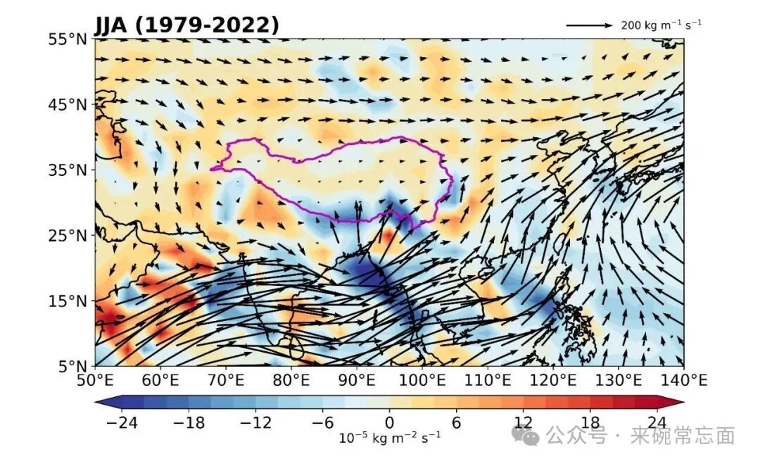 From the results, the most obvious feature is the significant summer monsoon water vapor transport process in South Asia and East Asia, corresponding to significant water vapor convergence regions in the western Indian subcontinent, eastern Bay of Bengal, southeastern Tibetan Plateau, and western Philippine Islands! Additionally, due to the influence of large topography, water vapor transport above the plateau is weak, while the results of direct integration from 1000 hPa show significant water vapor transport regions above the plateau, highlighting the importance of strictly starting integration from the surface!
4
Data Sources
- NCEP wind field and specific humidity data:
https://psl.noaa.gov/data/gridded/data.ncep.reanalysis.html
- Tibetan Plateau shp data:https://doi.org/10.11888/Geogra.tpdc.270099