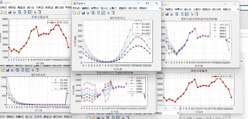
Using MATLAB to simulate the charging behavior of electric vehicles (EVs) through the Monte Carlo method, including conventional charging, fast charging, and battery swapping, and analyzing their impact on the daily load curve; unordered charging, controlled charging, controlled discharging curves, and their effects on the daily load curve. Reference documents attached.
 The following text and example code are for reference only.
Table of Contents
- 1. Preparation Phase
- 2. Model Construction
- 1. Define Parameters and Variables
- 2. Arrival Times and Charging Choices
- 3. Calculate Additional Load per Hour
- 4. Plot Results
- 3. Conclusion
To use MATLAB to simulate the charging behavior of electric vehicles (EVs), including conventional charging, fast charging, and battery swapping, and to analyze their impact on the daily load curve, we need to follow these steps. This process involves modeling various aspects: EV arrival patterns, charging behaviors, and the impact on grid load.
1. Preparation Phase
First, ensure you have the necessary toolbox, such as the Statistics and Machine Learning Toolbox for random number generation and other operations.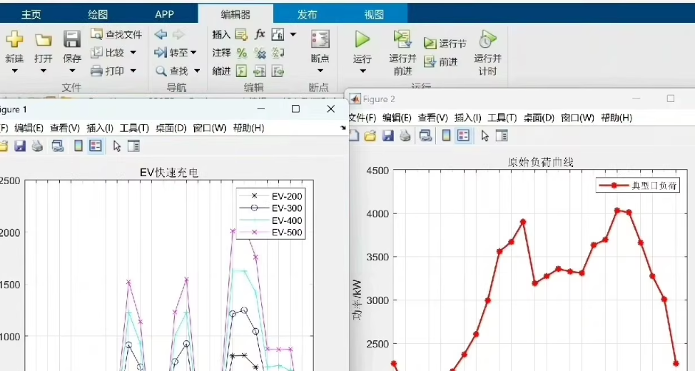
2. Model Construction
1. Define Parameters and Variables
- Number of Electric Vehicles: N
- Charging Power: Conventional charging (slow), fast charging, average power for battery swapping
- Charging Time Distribution: Based on historical data or assumptions
- Arrival Time Distribution: Can be assumed to follow a Poisson distribution or other suitable distributions
- Number of Hours in a Day: For example, 24 hours
% Parameter definition
N = 100; % Assume there are 100 electric vehicles
hours_in_day = 24;
slow_charge_power = 3.7; % kW, conventional charging power
fast_charge_power = 50; % kW, fast charging power
battery_swap_time = 0.5; % hours, time required for battery swapping
base_load = 1000; % kW, base load
2. Arrival Times and Charging Choices
We can use random numbers to simulate the arrival times of each vehicle and the choice of charging method.
rng(1); % Set random seed for reproducibility
arrival_times = poissrnd(60, [N, 1]); % Poisson distribution simulates arrival times
charging_types = randi([1, 3], [N, 1]); % 1: slow charge, 2: fast charge, 3: battery swap
charge_durations = zeros(N, 1);
for i = 1:N
    switch charging_types(i)
        case 1
            charge_durations(i) = unifrnd(4, 8); % Slow charge time 4 to 8 hours
        case 2
            charge_durations(i) = unifrnd(0.5, 1); % Fast charge time 0.5 to 1 hour
        case 3
            charge_durations(i) = battery_swap_time;
    end
end
3. Calculate Additional Load per Hour
Based on each vehicle’s arrival time and charging type, calculate the additional load for each hour.
load_profile = zeros(hours_in_day, 1);
for i = 1:N
    start_hour = mod(arrival_times(i), hours_in_day) + 1;
    end_hour = min(start_hour + floor(charge_durations(i)), hours_in_day);
    for hour = start_hour:end_hour
        if charging_types(i) == 1 || charging_types(i) == 2
            load_profile(hour) = load_profile(hour) + ...
                (charging_types(i) == 1) * slow_charge_power + ...
                (charging_types(i) == 2) * fast_charge_power;
        else
            load_profile(hour) = load_profile(hour) + fast_charge_power; % Assume battery swap station consumes the same as fast charge
        end
    end
end
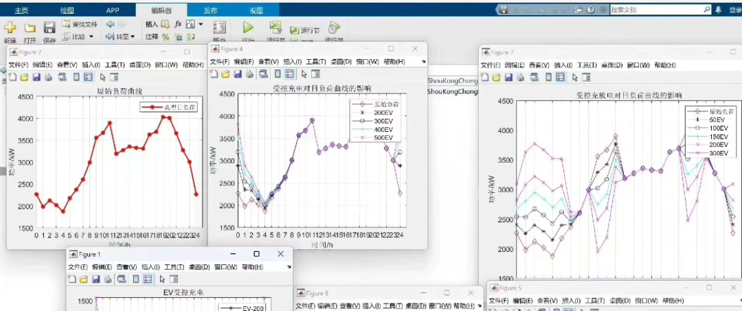
4. Plot Results
Finally, add the base load to the additional load caused by electric vehicle charging and plot the daily load curve.
total_load = base_load + load_profile;
figure;
plot(1:hours_in_day, total_load, '-o');
xlabel('Time (hours)');
ylabel('Total Load (kW)');
title('Daily Load Curve with Electric Vehicle Charging');
grid on;
3. Conclusion
The above code provides a basic framework to simulate different types of electric vehicle charging behaviors and their impact on the daily load curve of the power grid. You can adjust parameters such as the number of electric vehicles, the proportion of different types of charging, and charging power to better reflect the situation in specific scenarios.