A Real Python Project Experience

Copyright Statement: This article is an original work by the author, following the CC 4.0 BY-SA copyright agreement. Please include the original source link and this statement when reprinting.

Article link:

https://blog.csdn.net/lland5201314/article/details/117606268

Last weekend, I received a project worth 1200, with a 10% commission taken by the customer service, leaving me with 1000. I completed it in two hours and felt quite pleased. Such projects are actually rare; they have low technical difficulty but high prices, which we colloquially refer to as “easy money”. I thought about treating my goddess to a meal, but was ruthlessly rejected!

Effect Display

Tool Preparation

Data Source: https://maoyan.com/board/4?offset=1
Development Environment: Windows 10, Python 3.7
Development Tools: PyCharm, Chrome

Project Thought Analysis

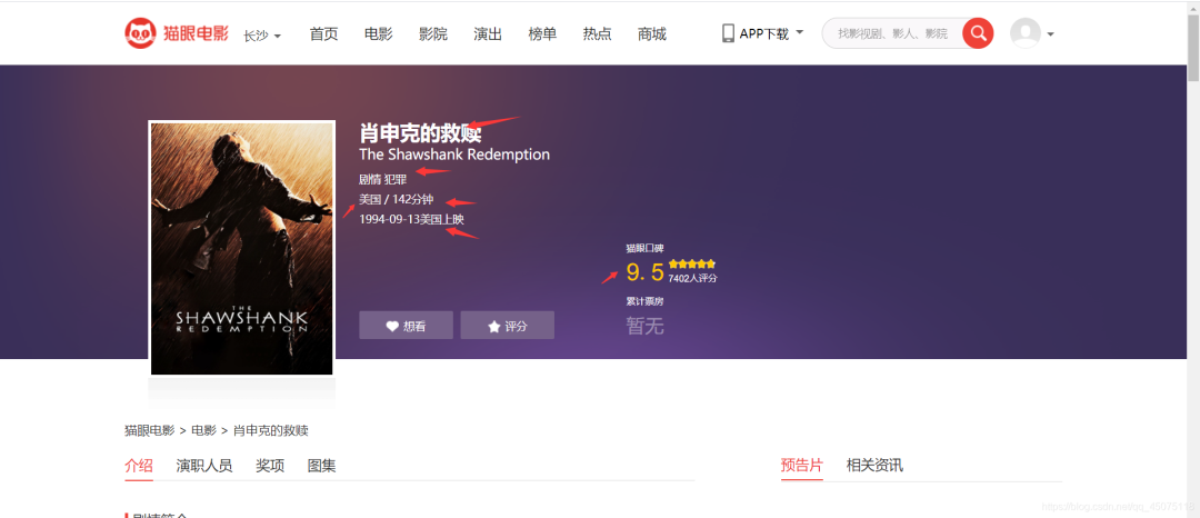
First, we need to collect all movie information from Maoyan. Here, we take the top 100 list as an example to obtain movie information:

Movie Name
Movie Rating
Movie Link
Movie Genre
Movie Release Location
Location
Movie Duration
Movie Duration

Parsing web data information

Parsing the homepage redirect links

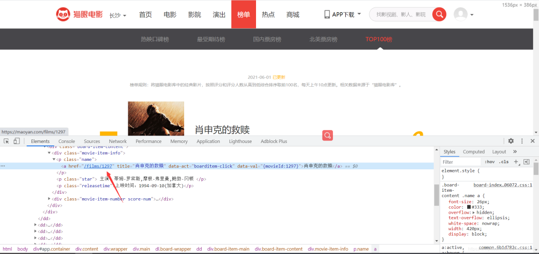The rating on the Maoyan detail page is encrypted, so we directly extract the rating information from the homepage.

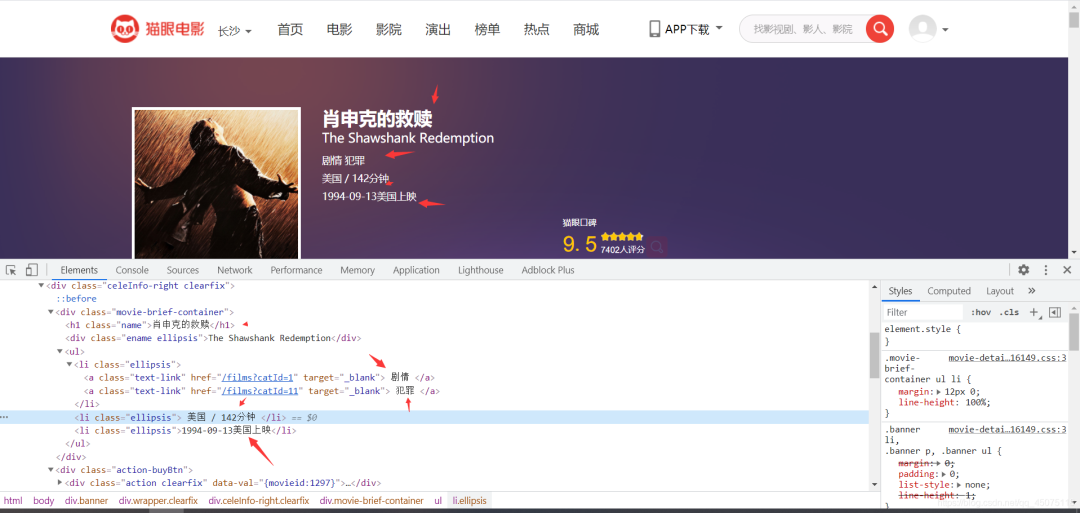
Extracting data from the detail page

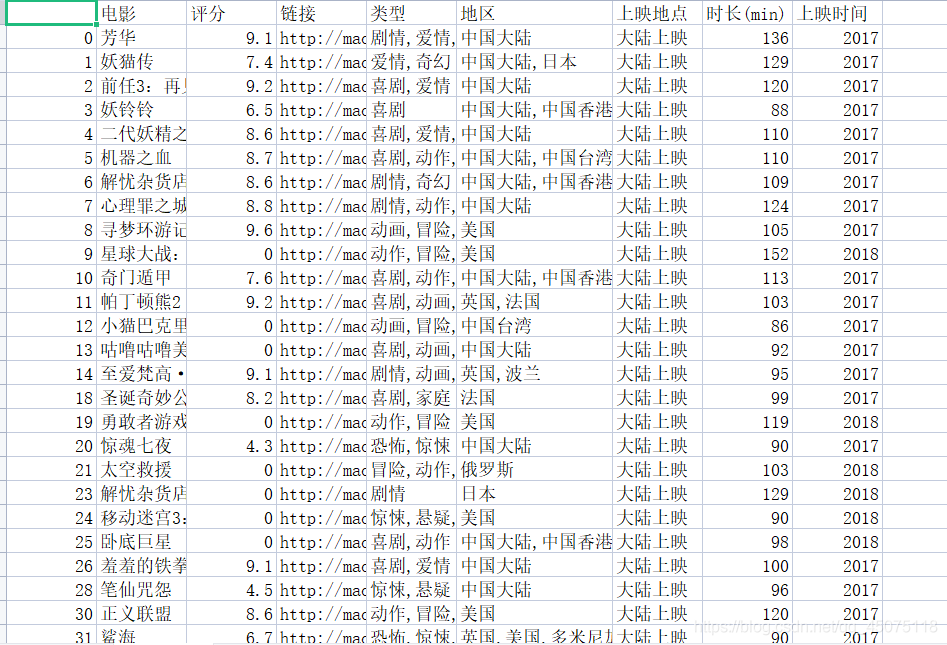
Save the data in a CSV file for easier data visualization later.

Tools Needed for Data Visualization

import pandas as pd
import numpy as np
import jieba
from wordcloud import WordCloud
import matplotlib.pyplot as plt
# get_ipython().run_line_magic('matplotlib', 'inline')

Effect Diagram Display

Source Code Display:

Web Crawler:

#!/usr/bin/env python
# -*- coding: utf-8 -*-
# @Time    : 2021-06-05
# @File    : demo4.py
import requests
from fake_useragent import UserAgent
from lxml import etree
import time

# Random request header
ua = UserAgent()

# Build request. You need to change it on the webpage. If you can't request, refresh the webpage and solve the captcha.
headers = {    'Accept': 'text/html,application/xhtml+xml,application/xml;q=0.9,image/webp,image/apng,*/*;q=0.8,application/signed-exchange;v=b3;q=0.9',    'Cookie': '__mta=244176442.1622872454168.1622876903037.1622877097390.7; uuid_n_v=v1; uuid=6FFF6D30C5C211EB8D61CF53B1EFE83FE91D3C40EE5240DCBA0A422050B1E8C0; _csrf=bff9b813020b795594ff3b2ea3c1be6295b7453d19ecd72f8beb9700c679dfb4; Hm_lvt_703e94591e87be68cc8da0da7cbd0be2=1622872443; _lxsdk_cuid=1770e9ed136c8-048c356e76a22b-7d677965-1fa400-1770e9ed136c8; _lxsdk=6FFF6D30C5C211EB8D61CF53B1EFE83FE91D3C40EE5240DCBA0A422050B1E8C0; ci=59; recentCis=59; __mta=51142166.1622872443578.1622872443578.1622876719906.2; Hm_lpvt_703e94591e87be68cc8da0da7cbd0be2=1622877097; _lxsdk_s=179dafd56bf-06d-403-d81%7C%7C12',    'User-Agent': str(ua.random)}

def RequestsTools(url):    '''    Crawler request tool function    :param url: Request address    :return: HTML object for xpath extraction    '''    response = requests.get(url, headers=headers).content.decode('utf-8')    html = etree.HTML(response)    return html

def Index(page):    '''    Homepage function    :param page: Page number    :return:    '''    url = 'https://maoyan.com/board/4?offset={}'.format(page)    html = RequestsTools(url)    # Detail page address suffix    urls_text = html.xpath('//a[@class="image-link"]/@href')    # Rating    pingfen1 = html.xpath('//i[@class="integer"]/text()')    pingfen2 = html.xpath('//i[@class="fraction"]/text()')
    for i, p1, p2 in zip(urls_text, pingfen1, pingfen2):        pingfen = p1 + p2        urs = 'https://maoyan.com' + i        # Avoid too frequent requests        time.sleep(2)        Details(urs, pingfen)

def Details(url, pingfen):    html = RequestsTools(url)    dianyan = html.xpath('//h1[@class="name"]/text()') # Movie name    leixing = html.xpath('//li[@class="ellipsis"]/a/text()') # Genre    diqu = html.xpath('/html/body/div[3]/div/div[2]/div[1]/ul/li[2]/text()') # Read total    timedata = html.xpath('/html/body/div[3]/div/div[2]/div[1]/ul/li[3]/text()') # Time    for d, l, b, t in zip(dianyan, leixing, diqu, timedata):        countyr = b.replace('\n', '').split('/')[0] # Location        shichang = b.replace('\n', '').split('/')[1] # Duration        f = open('猫眼.csv', 'a')        f.write('{}, {}, {}, {}, {}, {}, {}
'.format(d, pingfen, url, l, countyr, shichang, t))        print(d, pingfen, url, l, countyr, shichang, t)

for page in range(0, 11):    page *= 10    Index(page)

Visualization

#!/usr/bin/env python
# coding: utf-8
# Load commonly used data analysis libraries
import pandas as pd
import numpy as np
import jieba
from wordcloud import WordCloud
import matplotlib.pyplot as plt
# get_ipython().run_line_magic('matplotlib', 'inline')

# In[3]:

path='./maoyan.csv'
df=pd.read_csv(path,sep=',',encoding='utf-8',index_col=False)
df.drop(df.columns[0],axis=1,inplace=True)
df.dropna(inplace=True)
df.drop_duplicates(inplace=True)
df.head(10)


# Check the structure of the data
df.info()
print(df.columns)


# In[11]:

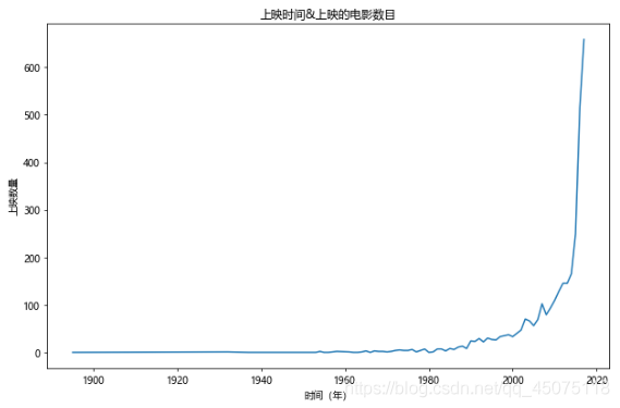
# Year & Number of Movies Released  The number of releases after 2018 is uncertain, so we will exclude them for now.
fig,ax=plt.subplots(figsize=(9,6),dpi=70)
df[df[u'上映时间']&lt;2018][u'上映时间'].value_counts().sort_index().plot(kind='line',ax=ax)
ax.set_xlabel(u'Year')
ax.set_ylabel(u'Number of Releases')
ax.set_title(u'Release Year & Number of Movies Released')


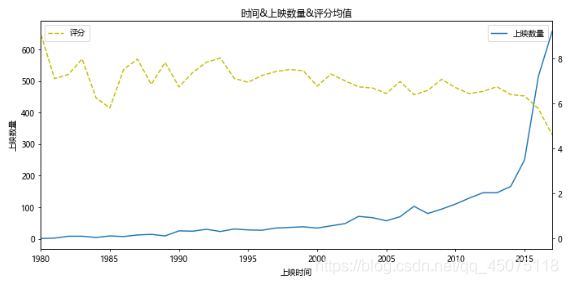
# Based on the above graph, create another graph showing the relationship between release year, number of releases, and ratings.
# However, due to the small amount of data before 1980, the ratings are inaccurate, so the main analysis area will focus on 1980-2017.
x=df[df[u'上映时间']&lt;2018][u'上映时间'].value_counts().sort_index().index
y=df[df[u'上映时间']&lt;2018][u'上映时间'].value_counts().sort_index().values
y2=df[df[u'上映时间']&lt;2018].sort_values(by=u'上映时间').groupby(u'上映时间').mean()[u'评分'].values
fig,ax=plt.subplots(figsize=(10,5),dpi=70)
ax.plot(x,y,label=u'Number of Releases')
ax.set_xlim(1980,2017)
ax.set_xlabel(u'Release Year')
ax.set_ylabel(u'Number of Releases')
ax.set_title(u'Release Year & Number of Releases & Average Ratings')
ax2=ax.twinx()
ax2.plot(x,y2,c='y',ls='--',label=u'Ratings')
ax.legend(loc=1)
ax2.legend(loc=2)

# Solve Chinese garbled characters and the issue of negative values not displaying on the axes.
plt.rcParams['font.sans-serif'] =['Microsoft YaHei']
plt.rcParams['axes.unicode_minus'] = False

# In[12]:

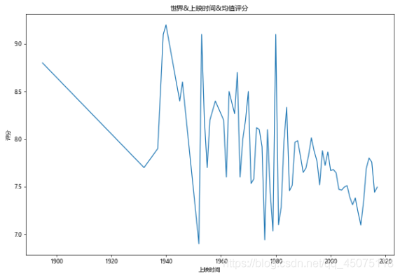
# World & Release Year & Average Ratings
fig,ax=plt.subplots(figsize=(10,7),dpi=60)
df[df[u'评分']&gt;0].groupby(u'上映时间').mean()[u'评分'].plot(kind='line',ax=ax)
ax.set_ylabel(u'Ratings')
ax.set_title(u'World & Release Year & Average Ratings')

# In[13]:

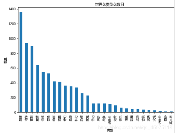
# Number of Movies by Genre Worldwide
# Split genres into the smallest units and then count.
types=[]
for tp in df[u'类型']:
    ls=tp.split(',')
    for x in ls:
        types.append(x)
tp_df=pd.DataFrame({u'类型':types})
fig,ax=plt.subplots(figsize=(9,6),dpi=60)
tp_df[u'类型'].value_counts().plot(kind='bar',ax=ax)
ax.set_xlabel(u'Genre')
ax.set_ylabel(u'Number')
ax.set_title(u'World & Genre & Number')

# In[14]:

# Distribution of Movie Duration and Ratings
# There is an issue: some movies have not been rated, so we need to exclude those.
x=df[df[u'评分']&gt;0].sort_values(by=u'时长(min)')[u'时长(min)'].values
y=df[df[u'评分']&gt;0].sort_values(by=u'时长(min)')[u'评分'].values
fig,ax=plt.subplots(figsize=(9,6),dpi=70)
ax.scatter(x,y,alpha=0.6,marker='o')
ax.set_xlabel(u'Duration (min)')
ax.set_ylabel(u'Number')
ax.set_title(u'Distribution of Movie Duration & Ratings')
# You can see the ratings.

i=0
c0=[]
c1=[]
c2=[]
c3=[]
c4=[]
c5=[]
c6=[]
c7=[]
for x in df[u'地区']:
    if u'中国大陆' in x:
        c0.append(df.iat[i, 0])
        c1.append(df.iat[i, 1])
        c2.append(df.iat[i, 2])
        c3.append(df.iat[i, 3])
        c4.append(df.iat[i, 4])
        c5.append(df.iat[i, 5])
        c6.append(df.iat[i, 6])
        c7.append(df.iat[i, 7])
    i=i+1
china_df=pd.DataFrame({u'电影':c0, u'评分':c1,u'链接':c2, u'类型':c3,u'地区':c4, u'上映地点':c5,u'时长(min)':c6,u'上映时间':c7})

# In[16]:

# Comparison of Average Ratings between China & the World for the Time Range 1980-2017
x1 = df[df[u'评分']&gt;0].groupby(u'上映时间').mean()[u'评分'].index
y1 = df[df[u'评分']&gt;0].groupby(u'上映时间').mean()[u'评分'].values    
x2 = china_df[china_df[u'评分']&gt;0].groupby(u'上映时间').mean()[u'评分'].index
y2 = china_df[china_df[u'评分']&gt;0].groupby(u'上映时间').mean()[u'评分'].values
fig,ax=plt.subplots(figsize=(12,9),dpi=60)
ax.plot(x1,y1,ls='-',c='DarkTurquoise',label=u'World')
ax.plot(x2,y2,ls='--',c='Gold',label=u'China')
ax.set_title(u'Average Ratings Comparison between China & the World')
ax.set_xlabel(u'Time')
ax.set_xlim(1980,2017)
ax.set_ylabel(u'Ratings')
ax.legend()

# In[17]:

# Number of Movies by Genre: Comparison between China & the World
# Since genres are mixed, to facilitate statistics, first write a function to split genres.

# In[18]:

# Function to split genres: Pass in a Series type object and return a DataFrame with split genres.
# Here we pass in a Series of genres.
def Cuttig_type(typeS):    types=[]    types1=[]
    for x in typeS:        if len(x)&lt;4:            # print x            types1.append(x)        ls=x.split(',')        for i in ls:            types.append(i)
    types.extend(types1)    df=pd.DataFrame({u'类型':types})    return pd.DataFrame(df[u'类型'].value_counts().sort_values(ascending=False))

# In[19]:

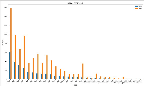
# Comparison of Movie Types between China & the World
df1=Cuttig_type(china_df[u'类型'])
df2=Cuttig_type(df[u'类型'])
trans=pd.concat([df1,df2],axis=1)
trans.dropna(inplace=True)
trans.columns=[u'中国',u'世界']
fig,ax=plt.subplots(figsize=(15,9),dpi=80)
trans.plot(kind='bar',ax=ax) 
fig.autofmt_xdate(rotation=30)
ax.set_title(u'Comparison of Movie Types between China & the World')
ax.set_xlabel(u'Genre')
ax.set_ylabel(u'Number of Movies')

# In[20]:

# Then we have the scatter distribution: China & the World & Duration & Ratings distribution.
y = df[df[u'评分'] &gt; 0].sort_values(by=u'时长(min)')[u'评分'].values
x = df[df[u'评分'] &gt; 0].sort_values(by=u'时长(min)')[u'时长(min)'].values
y2 = china_df[china_df[u'评分'] &gt; 0].sort_values(by=u'时长(min)')[u'评分'].values
x2 = china_df[china_df[u'评分'] &gt; 0].sort_values(by=u'时长(min)')[u'时长(min)'].values
fig, ax = plt.subplots(figsize=(10,7), dpi=80)
ax.scatter(x, y, c='DeepSkyBlue', alpha=0.6, label=u'World')
ax.scatter(x2, y2, c='Salmon', alpha=0.7, label=u'China')
ax.set_title(u'Distribution of Ratings between China & the World')
ax.set_xlabel(u'Duration (min)')
ax.set_ylabel(u'Ratings')
ax.legend(loc=4)

# In[25]:

dfs=df[(df[u'上映时间']&gt;1980)&amp;(df[u'上映时间']&lt;2019)]


# for x in range(0,len(dfs)):#     print(dfs.iat[x,0],dfs.iat[x,-1])
df666 = dfs['电影'][:15]
wl = ",".join(df666.values)# Write the segmented words into a text file# fenciTxt  = open("fenciHou.txt","w+")# fenciTxt.writelines(wl)# fenciTxt.close()
# Set up the word cloud
lwc = WordCloud(background_color="white",  # Set background color               # mask=imread('shen.jpg'),   # Set background image#                    max_words=2000,  # Set maximum number of words to display                   font_path="C:\Windows\Fonts\simkai.ttf", # Set to KaiTi Regular    # Set Chinese font to display (the default font for word cloud is "DroidSansMono.ttf", which does not support Chinese)               max_font_size=60, # Set maximum font size               random_state=30,  # Set how many random generation states, i.e., how many color schemes               )
myword = wc.generate(wl)  # Generate word cloud
wc.to_file('result.jpg')
# Display word cloud
plt.imshow(myword)
plt.axis("off")
plt.show()

# In[41]:

Conclusion

The source code has been provided, so I won’t analyze it. If it is useful to everyone, please give it a thumbs up, thank you very much. Finally, let me show you my project experience.

PS: Always use a third-party platform for project orders!!! PS: Always use a third-party platform for project orders!!! PS: Always use a third-party platform for project orders!!!

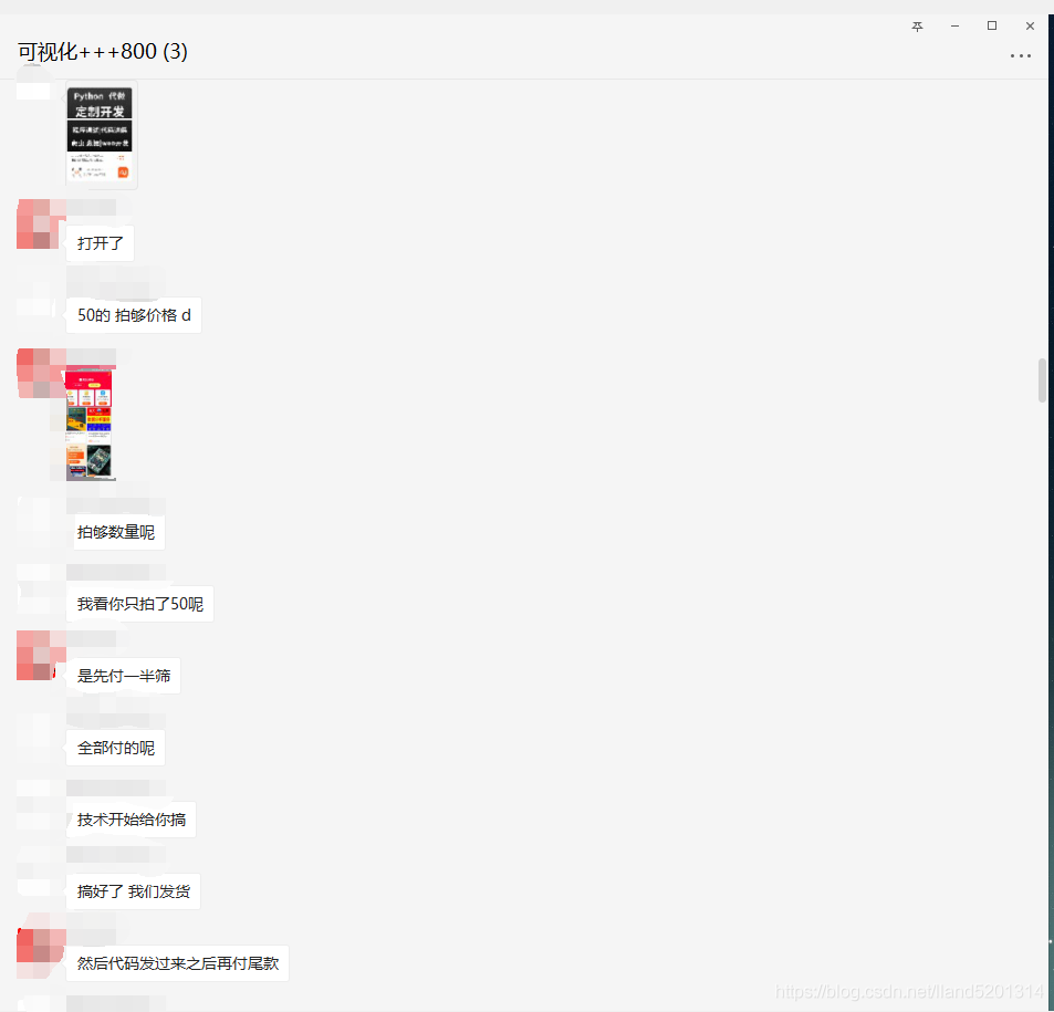
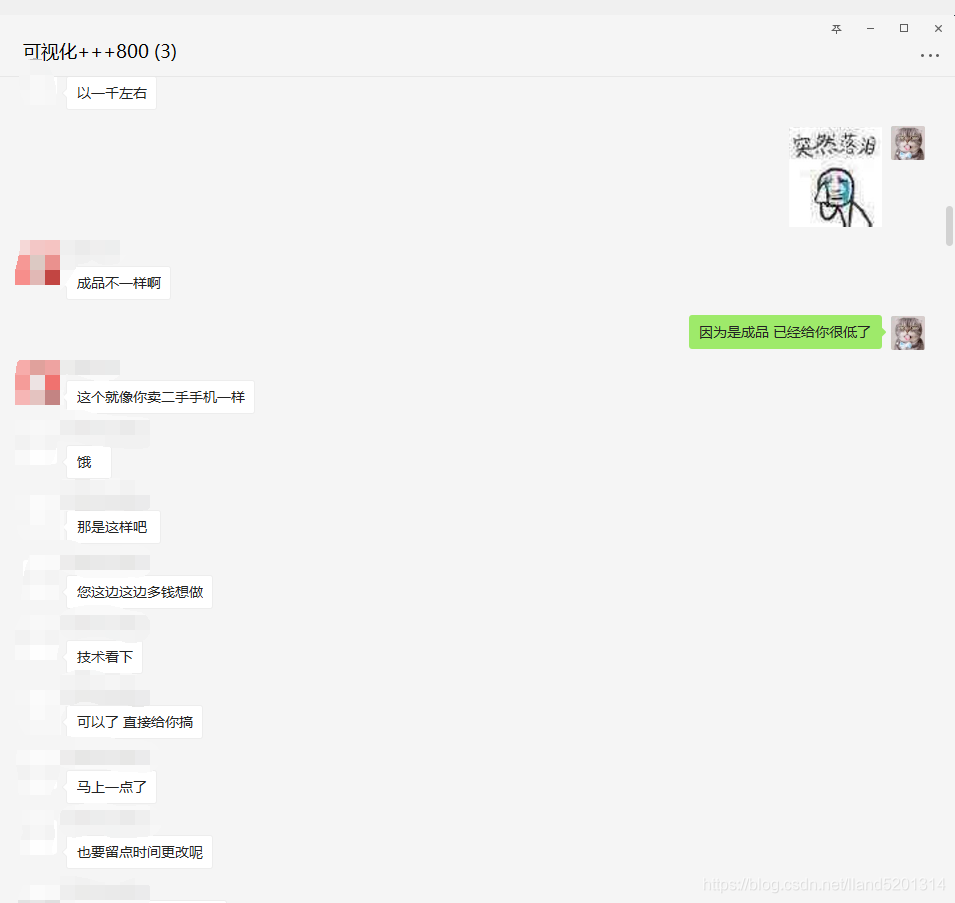
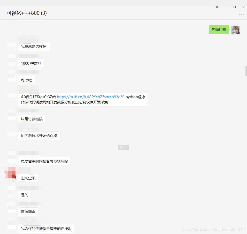
PS: Always use a third-party platform for project orders!!!PS: Always use a third-party platform for project orders!!!PS: Always use a third-party platform for project orders!!!