DTI imaging has a relatively long application history, as it can display the overall orientation of fiber bundles and generate quantitative parameters such as FA values and MD values to reflect microstructural information. However, studies have shown that this model has limitations in displaying complex fiber bundle orientations, especially for crossing fibers and fibers with branching structures.
To better display the structural characteristics of complex fiber bundles and accurately determine their orientations, researchers have proposed different methods, such as the well-known diffusion spectrum imaging (diffusion spectrum imaging, DSI)(Figure 1). Siemens’ “MAGNETOM Prisma” with its powerful research performance is the only device in the industry capable of achieving 15 minutes of whole-brain DSI diffusion spectrum imaging (whereas conventional 3T imaging under the same conditions requires over 45 minutes), accurately displaying the crossing, intertwining, segmentation, and termination of neural fiber bundles, which is of great significance for clinical and research applications in the nervous system.。
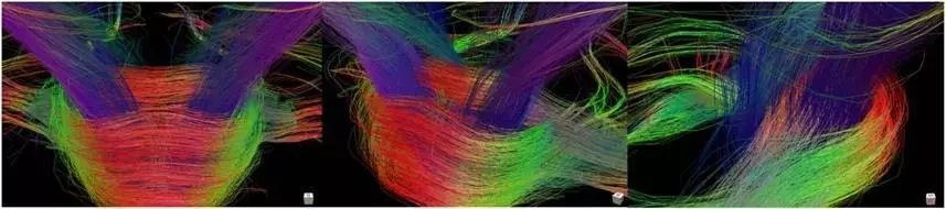
Figure 1. Fiber bundle images reconstructed using the DSI algorithm with partial grid data (grid sampling)(514 points).
In fact, DSI is just one of the methods for displaying complex fiber bundle orientations. There are also the well-known q-ball imaging (q-ball imaging, QBI) and generalized q-sampling (Generalized q-Sampling, GQI)(Figure 2). To better understand these different post-processing models, let’s start with the basic concepts involved.
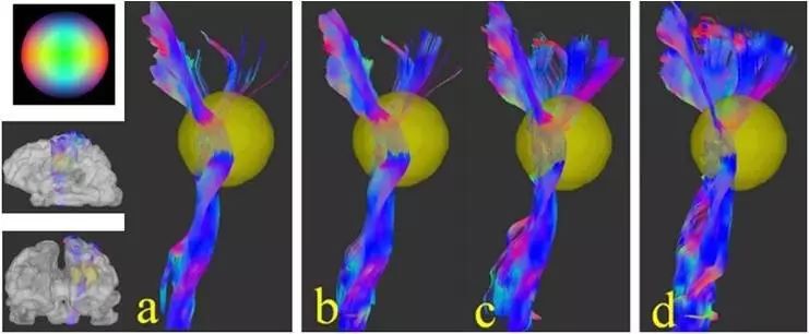
Figure 2. Reconstructed fiber bundle images, (a) using the QBI reconstruction model with 252 direction shell data (shell dataset), (b) reconstruction using the GQI model with the same data type, (c) reconstruction results based on 203 point grid data (grid sampling) using the DSI model, (d) results reconstructed with the same data using the GQI model.
1. Q-Space Imaging
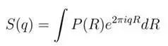
The reason for introducing the concept of “q-space” imaging is that it serves as the foundation for advanced reconstruction algorithms for fiber bundles. Whether it is DSI, QBI, or GQI, they are essentially different post-reconstruction algorithms based on q-space data (Figure 3). So what is “q-space” imaging? “q-space” imaging was proposed by Callaghan in 1994. To better understand this concept, we can compare it with “K-space” in MR imaging. The data encoding in K-space is achieved using frequency encoding gradients (readout gradient), while the encoding in q-space is accomplished using diffusion encoding gradients. Data in K-space can be associated with the spatial location of hydrogen protons through Fourier transform, while data in q-space can yield a dataset known as the “ensemble average propagator (ensemble average propagator, EAP)” through Fourier transform. The relationship between them can be expressed as follows:
“q-space “ imaging assesses the diffusion motion of hydrogen protons in relation to the EAP. So what is EAP? In simple terms, it is a three-dimensional probability density function of hydrogen proton displacement. The term “average” indicates that this factor is merely an average assessment of the diffusion of hydrogen protons within the tissue, without considering the heterogeneity of the tissue, while “displacement” indicates that this factor assesses the relative displacement of hydrogen protons, not their absolute positions. Therefore, “q-space” imaging is a non-parametric method for studying diffusion motion.q is defined as follows:q=γGδ/2π, b=(2π)2Δ From this, we can see that a higher q bandwidth can lead to greater sensitivity in displacement detection.R。
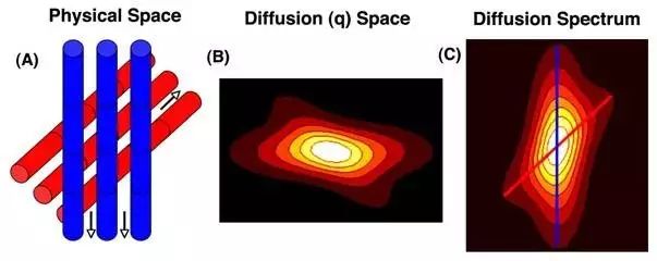
Figure 3. Illustration of the actual arrangement direction of the object and “q-space” imaging. Source: Sosnovik, D. E., Wang, R., Dai, G., Reese, T. G., & Wedeen, V.J. (2009). Diffusion MR tractography of the heart. Journal of Cardiovascular Magnetic Resonance, 11(1), 1-15.
2. Diffusion Sampling Scheme
The reason for introducing the “Diffusion Sampling Scheme” is that different fiber bundle reconstruction models have different requirements for sampling data. For example, the QBI model requires the data collection scheme to be shell data (shell dataset), the DSI model requires the data collection scheme to be grid data (grid sampling), while the GQI model can apply to both types of data sampling schemes.Diffusion-weighted images can be achieved using a series of different diffusion-sensitive encoding gradients. The classification of diffusion data sampling schemes is based on the spatial distribution of the gradient encoding vectors (Gx, Gy, Gz) and can be divided into three categories: single-shell data (Single-shell dataset), multi-shell data (Multi-shell dataset), and grid data sampling schemes (grid sampling scheme)(Figure 4):
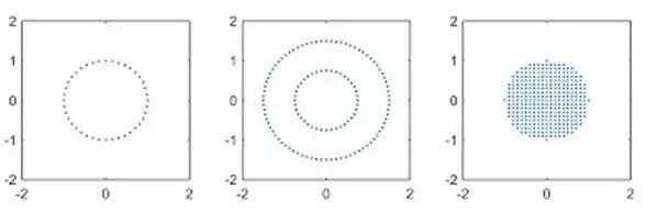
Figure 4. From left to right, single-shell data (Single-shell dataset), multi-shell data (Multi-shell dataset), and grid data sampling scheme illustration.
3. Diffusion Orientation Distribution Function (dODF)
The reason for introducing this function is that it is the basis for the reconstruction of the QBI and DSI models. Only by first calculating the function value of this function can we further perform tracking analysis of complex fiber bundles. This function is also a method for analyzing the DSI model’s EAP factor.
By projecting the EAP (3D PDF) onto a unit sphere, we can calculate the diffusion orientation distribution function (diffusion orientation distribution function, dODF) values (Figure 5), which reflects the probability distribution of the diffusing hydrogen protons within the unit sphere. It is important to note that there are multiple methods to achieve this projection, and common methods for calculating dODF are as follows:
1. Unweighted No Upper Limit dODF, function as follows:
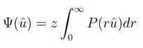
This psi function is the dODF function, where u is the unit vector of direction, P is the EAP, and r is the displacement of hydrogen protons.
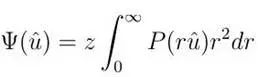
2. r Squared Weighted No Upper Limit dODF, function as follows:
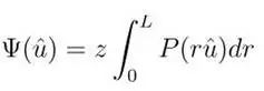
3. Unweighted With Upper Limit dODF, function as follows:
The QBI, DSI, and GQI respectively adopt different methods to calculate dODF, where QBI uses the unweighted no upper limit dODF, DSI applies the r squared weighted no upper limit dODF, and GQI applies unweighted or r squared weighted upper limit dODF. To calculate dODF, QBI often uses the Funk-Radon transform to compute dODF. The DSI requires first performing an inverse Fourier transform to obtain the EAP, and then integrating the EAP to obtain dODF, but usually, the EAP has a high noise level, so during the reconstruction process, Hanning filtering is often needed for smoothing.
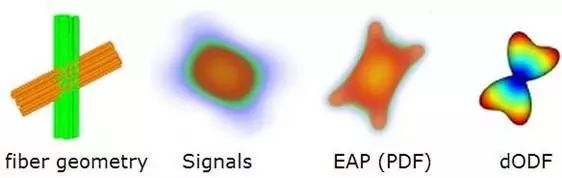
Figure 5. Illustration of crossing fiber orientation and corresponding EAP and dODF images.
4. Hydrogen Proton Distribution Function (Spin Distribution Function, SDF)
The reason for introducing this function is that it serves as the basis for the reconstruction of the GQI model. Using this function, GQI can apply to any diffusion-weighted data collection scheme (e.g. DTI, DSI, HARDI, multishell), and can also evaluate diffusion-restricted information.
dODF is a probability density function; if we weight this function by hydrogen proton density, we can obtain the hydrogen proton distribution function in different directions. In fact, this is also the theoretical basis of the GQI model, which directly computes the signal from q-space to obtain the SDF, with the mathematical model as follows:
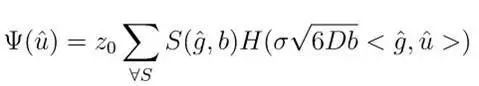
Z0 is a constant that normalizes the tissue hydrogen proton density based on the hydrogen content of water; S: diffusion signal intensity; b:b value; sigma: upper limit of diffusion distance; H(.): is a basis function, H(.) uses the sinc function to convert the SDF into a form of ODF without weight (also known as GQI0, unweighted form of GQI). Different basis functions can also be used to compute GQI1 (r weighted) and GQI2 (r squared weighted). It is worth noting that since the SDF is weighted using hydrogen protons, it can be considered as a resampling of hydrogen proton density in the radial direction. This gives the function a quantifiable role, rather than just being a probability density function. Specifically, the SDF function quantifies the density of diffusing hydrogen protons with a displacement less than L in the direction of u. This is different from the QBI and DSI models, which apply the dODF function, as the latter is merely a probability function, where the sum in all directions can only equal 1. In the axial direction, the quantity of hydrogen proton diffusion can be represented by quantitative anisotropy (quantitative anisotropy, QA), and the parameter sigma allows us to calculate the radial diffusion information and diffusion-restricted information at any length.
Earlier, we introduced the common data collection schemes in q-space imaging, along with the basic concepts involved in advanced reconstruction algorithms, where single-shell data is most sensitive to direction, while grid data evenly encompasses both organizational direction and radial information. If a study is only concerned with axial direction, single-shell data is the most efficient sampling scheme; if a study involves changes in tissue pathology, the grid data sampling scheme is the best choice, as it comprehensively considers both directional and radial information.
In the next issue, we will provide a brief overview of complex reconstruction models and introduce quantitative analysis metrics that can be used in analyzing q-space data for clinical reference (The above content is translated from www.dsi-studio.labsolver.org/).
References:
[1] Callaghan, P.T., Principles of Nuclear Magnetic Resonance Microscopy. 1994: Oxford University Press.
[2] Tuch, David S. “Q‐ball imaging.” Magnetic Resonance in Medicine 52.6 (2004): 1358-1372.
[3] Wedeen, Van J., et al. “Mapping complex tissue architecture with diffusion spectrum magnetic resonance imaging.” Magnetic Resonance in Medicine 54.6 (2005): 1377-1386.
[4] Yeh, Fang-Cheng, Van Jay Wedeen, and Wen-Yih Isaac Tseng. “Generalized-sampling imaging.” Medical Imaging, IEEE Transactions on 29.9 (2010): 1626-1635.
[5] Barnett, Alan. “Theory of Q‐ball imaging redux: Implications for fiber tracking.” Magnetic Resonance in Medicine 62.4 (2009): 910-923.
[6] Fang-Cheng Yeh, Van Jay Wedeen, and Wen-Yih Isaac Tseng. Generalized-Sampling Imaging. IEEE TRANSACTIONS ON MEDICAL IMAGING, VOL. 29, NO. 9, SEPTEMBER 2010.
Click the button in the top right corner to share with friends and let more people know about the latest advancements in MRI.
Scan the QR code below to follow 【MRI Enthusiasts】