MLNLP community is a well-known machine learning and natural language processing community, with an audience covering NLP master’s and doctoral students, university professors, and corporate researchers.

The vision of the community is to promote communication and progress between the academic and industrial sectors of natural language processing and machine learning, especially for beginners.

Reprinted from | Zhihu

Author | Ran Di

1. How to estimate GPU memory usage during training and inference given the parameter count of a model?

2. Which part of memory is saved when using Lora compared to full parameter training? What about Qlora compared to Lora?

3. What is the specific process of mixed precision training?

This is a question I was asked in an interview. To consolidate the relevant knowledge, I plan to systematically write an article to help myself review for the autumn recruitment while hoping it can also help my fellow friends. This article will systematically analyze the GPU memory usage of large models during training or inference on a single GPU. Some knowledge points may not be explored too deeply (as I am not an expert), but I will try to ensure that the entire read is logically coherent and easy to understand (only a beginner understands a beginner best!).

1. Data Precision

To calculate GPU memory usage, we need to know the precision of the data we are using at the “atomic” level, as precision determines how data is stored and how many bits a piece of data occupies. We all know:

1 byte = 8 bits

1 KB = 1,024 bytes

1 MB = 1,024 KB

1 GB = 1,024 MB

From this, we can understand that a model with 1G parameters, if each parameter is 32 bits (4 bytes), will directly occupy 4x1G of GPU memory when loaded.

1.1 Common Precision Types

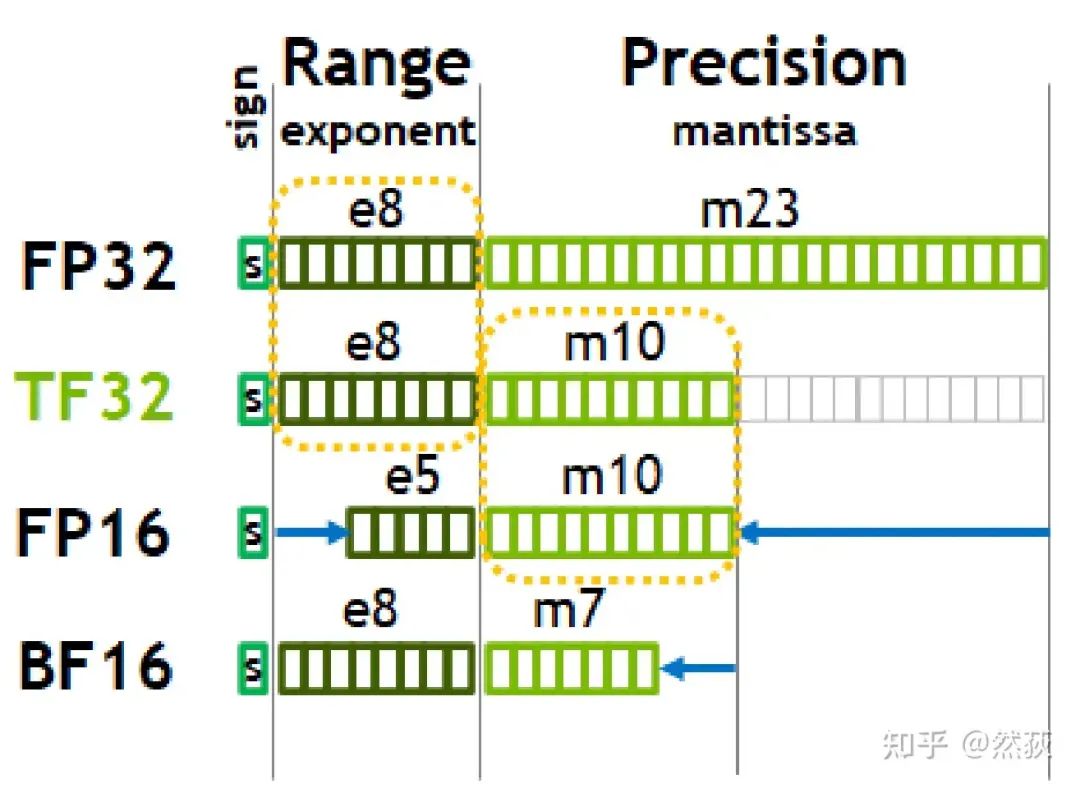
I believe it is enough to master the few common data types shown in the figure below. For more precision types, you can understand them by analogy. The figure is sourced from NVIDIA’s Ampere architecture white paper:

Understanding GPU Memory Usage in Large Models (Single GPU)

It can be very intuitively seen that floating-point numbers consist of three parts: the sign bit, the exponent, and the mantissa. The sign bit is 1 bit (0 for positive, 1 for negative), the exponent affects the range of the floating-point number, and the mantissa affects precision. Note that TF32 is not actually 32 bits; it is only 19 bits, so don’t confuse them. BF16 refers to Brain Float 16, proposed by the Google Brain team.

1.2 Specific Calculation Example

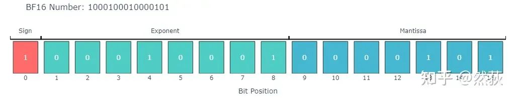
As a master’s student, I believe that showing a vivid image or example is more direct than lengthy explanations. Below we will use an example to deeply understand how to derive our final data from these three parts: I will take BF16, the most widely used precision type in the industry, as an example, and the numbers below are randomly generated by my friend Claude:

Problem:

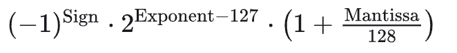
– First, provide the specific calculation formula:

– Then analyze step by step (not sure why I used Cot on myself)

Sign bit = 1, representing a negative number

Exponent = 17, the middle part is

Mantissa = 3, the latter part is

Final Result

The three parts multiplied together give the final result -8.004646331359449e-34

Notes

The only thing to note is that the all-zero and all-one states of the exponent are special cases and cannot be used in the formula. If you want to understand more deeply, you can refer to this blog: Thoroughly Understand the Calculation Method of float16 and float32 – CSDN Blog. If you are interested in learning more about how to convert from FP32 to BF16, you can check out this blogger’s explanation: Understanding FP16, BF16, TF32, FP32 from an Interview.

2. Memory Analysis of Full Parameter Training and Inference

Now that we know the storage method and size corresponding to data precision, it is equivalent to understanding the different specifications of machine parts in a factory, but we also need to understand the operation process of the entire production line to accurately estimate the resources (GPU memory) required when the entire factory (i.e., our model training process) is running. Let’s take the most common mixed precision training method as a reference to see where the GPU memory goes.

2.1 Mixed Precision Training

2.1.1 Principle Introduction

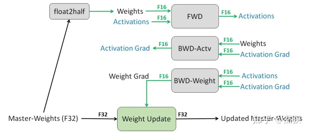
As the name suggests, mixed precision training involves mixing multiple different precision data during training. The paper “MIXED PRECISION TRAINING” combines FP16 and FP32, using the Adam optimizer, as shown in the figure below:

According to the logic of training operation:

Step 1: The optimizer first backs up a copy of the FP32 precision model weights and initializes the first and second-order momentum (used to update weights) in FP32 precision.

Step 2: Allocate a new storage space to convert the FP32 precision model weights to FP16 precision model weights.

Step 3: Run forward and backward passes, with the gradients and activation values all stored in FP16 precision.

Step 4: The optimizer updates the backed-up FP32 model weights using the FP16 gradients and FP32 first and second-order momentum.

Step 5: Repeat Steps 2 to 4 for training until the model converges.

We can see that during the training process, GPU memory is mainly used in four modules:

Model weights themselves (FP32 + FP16)
Gradients (FP16)
Optimizer (FP32)
Activation values (FP16)

2.1.2 Three Small Questions

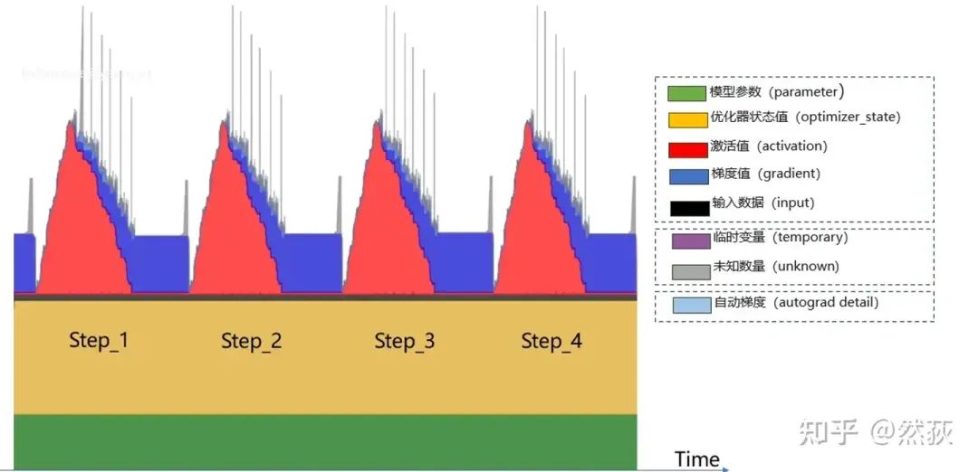
At this point, I have three small questions. The first question is, why not use FP16 for everything? Wouldn’t that make calculations faster and use less memory?

Based on our knowledge from the first chapter, we know that FP16 precision has a much narrower range than FP32, which can lead to two issues: data overflow and rounding errors (if you want to learn more, please refer to the most comprehensive guide on mixed precision training principles). This can result in gradient disappearance and inability to train, so we cannot use FP16 for everything; we still need FP32 for precision assurance. You might think that BF16 could replace FP16, and yes, that is also why many trainings today use BF16—at least BF16 does not produce data overflow, and industry feedback shows that larger models care more about range than precision.

The second question is, why do we only perform half-precision optimization on activation values and gradients while adding a new FP32 model copy? Wouldn’t that increase GPU memory usage?

The answer is no; activation values are related to batch size and sequence length, and in actual training, the activation values occupy a large amount of GPU memory. The positive optimization of activation values outweighs the negative optimization of the backup model parameters, resulting in reduced overall GPU memory. (Here, gradient checkpointing optimization methods can also be considered to further optimize the GPU memory of activation values; if interested, you can check out this foundational knowledge on efficient training of large models: Gradient Checkpointing).

The third question is, we know that GPU memory, like RAM, has static and dynamic distinctions. Which of the mentioned items are static and which are dynamic?

Most people can guess:

Static: Optimizer state, model parameters
Dynamic: Activation values, gradient values

In other words, we cannot accurately calculate the actual GPU memory size during operation. If this comes up in an interview, you can ignore the calculation of activation values and treat gradients as static calculations. If you want to explore deeply, I recommend [LLM] GPU Memory Calculation Formula and Optimization for Large Models.

2.1.3 Let’s Do a Test!

At this point, we should have no problem analyzing GPU memory issues during large model training (except for the dynamic part). So let’s conduct a real test; those reading can also try calculating it themselves to see if they truly understand. For the llama3.1 8B model, with FP32 and BF16 mixed precision training using the AdamW optimizer, what is the approximate GPU memory usage during model training?

Solution:

Model parameters: 16 (BF16) + 32 (PF32) = 48G

Gradient parameters: 16 (BF16) = 16G

Optimizer parameters: 32 (PF32) + 32 (PF32) = 64G

Ignoring activation values, the total GPU memory usage is approximately (48 + 16 + 64) = 128G

2.2 Inference and KV Cache

2.2.1 Understanding the Principles

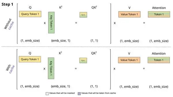
During inference, GPU memory mainly considers the model parameters themselves; in addition, the currently widely used KV cache also occupies GPU memory. The KV cache differs from the previously discussed methods of reducing memory; its purpose is to reduce latency, sacrificing memory for inference speed.

I won’t elaborate on what KV cache is; a dynamic image can clarify it very clearly (if still unclear, you can refer to Accelerating Large Model Inference: Learning KV Cache through Images). Remember, during inference, we are continuously performing the task of “generating the next token”. The generation of the current token only relates to the current QKV and all previous KVs, so we can maintain this KV and continuously update it.

By the way, let me answer a common question many beginners ask: why is there no Q cache?

Because generating the current token only depends on the current Q. Why does generating the current token only depend on the current Q? This is determined by the self-attention formula:

We can see that at position t in the sequence, i.e., the t-th row, it only relates to 𝑄𝑡, meaning the attention calculation formula determines that we do not need to save Q at each step. Furthermore, the mathematical properties of matrix multiplication dictate that we do not need to save Q at each step.

2.2.2 Calculating KV Cache Memory

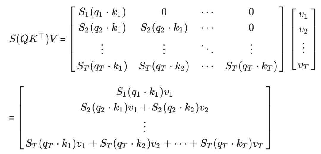
The calculation of KV cache memory is what I want to focus on in this article. Here is the formula:

The first four parameters multiplied should be easy to understand, as KV corresponds to the total of all hidden vectors in each layer of the model. The first 2 refers to the two parts of KV, and the second 2 refers to the byte size corresponding to half precision.

For example, for llama7B, with hiddensize = 4096, seqlength = 2048, batchsize = 64, layers = 32, the calculation yields:

It can be seen that in the case of large batches and long sentences, the GPU memory usage of the KV cache is also significant.

68G appears to be quite large relative to the model itself, but this is under a large batch condition. In a single batch, the KV cache occupies only about 1G of GPU memory, which is just half the memory of the model parameters.

2.2.3 MQA and GQA

What? You think the memory usage of the KV cache is still too high? For inference on the landing side, it is reasonable to impose strict requirements. MQA and GQA are methods used to further reduce memory usage, and most large models today use this method. Let’s talk about it.

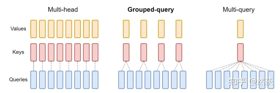
Actually, the methods are not hard to understand; the image makes it clear at a glance. The keyword is “shared multi-head KV”, which is a simple idea of removing redundant structures in the model. The leftmost is the basic MHA multi-head self-attention, the middle GQA retains several groups of KV heads, while the rightmost MQA retains only one group of KV heads. Currently, GQA is the most commonly used, as it reduces GPU memory and speeds up processing without significantly affecting performance. If you don’t understand, you can refer to Accelerating Large Model Inference: Detailed Look at KV Cache and GQA; I won’t elaborate here, but I want to discuss the specific changes in memory usage.

In the previous section, we learned that the memory usage calculation formula for MHA’s KV cache is:

A small detail is that you can start training MQA and GQA models from scratch, or you can modify the model structure based on open-source models as in the GQA paper and continue pre-training. Currently, most are trained from scratch to ensure consistency between the training and inference model structures.

3. Memory Analysis of Lora and Qlora

In the previous two chapters, we detailed the memory analysis of full parameter fine-tuning training and inference. Smart readers have noticed a problem: nowadays we use PEFT (Parameter-Efficient Fine-Tuning), who has the resources for full parameter training? Inference also needs quantization, so how should we conduct memory analysis? In this chapter, we will solve this problem. I believe that those who fully understand the previous two chapters will find it very easy to understand. The so-called memory analysis can be done similarly as long as we know the specific process and data precision. OK, we will analyze the memory usage of the currently most popular Lora and Qlora methods in detail in this chapter, and relevant principle knowledge will also be involved. Let’s go!

3.1 Lora

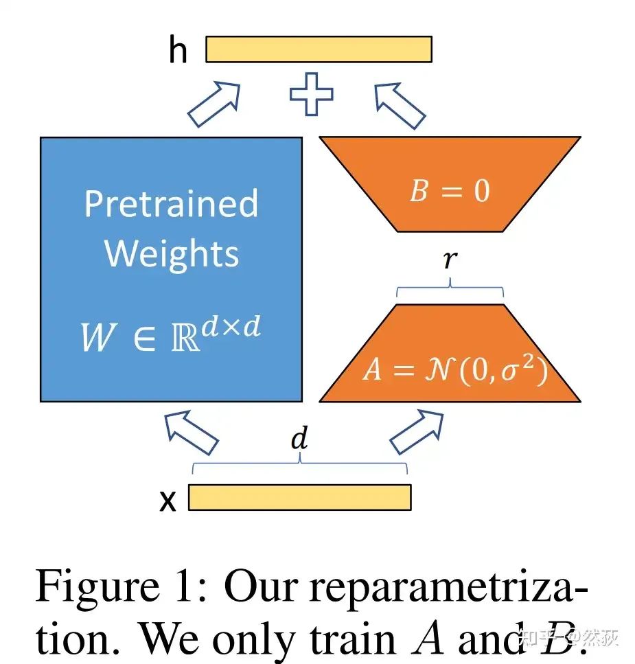
Those who can see this must have a good understanding of Lora’s principles. Briefly, as shown in the figure below, a pair of low-rank trainable weights is created alongside the original weight matrix; during training, only the side path is trained, greatly reducing the number of weights trained, reducing the parameter count from d*d to 2*d*r.

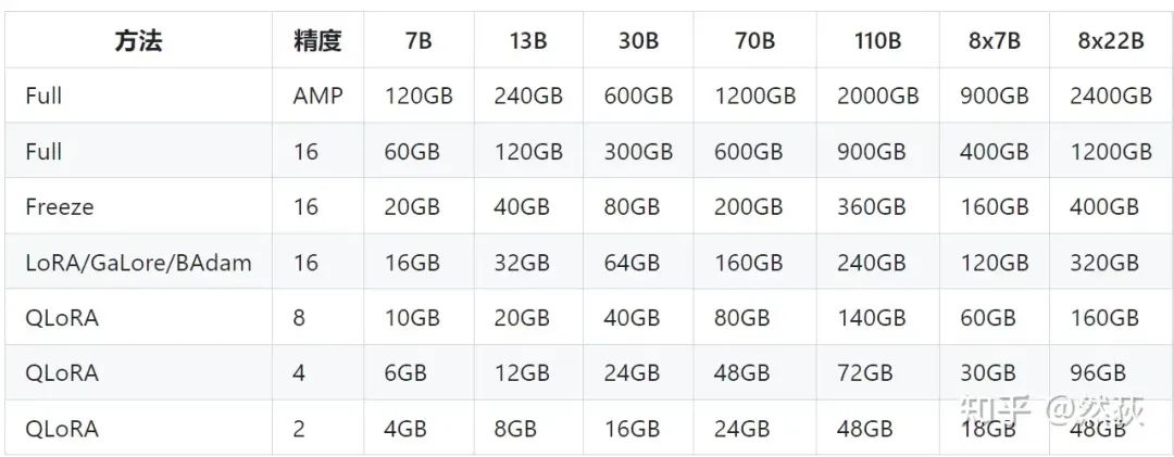
With the previous full parameter training memory analysis, the analysis is quite smooth. Let’s go step by step, still using BF16 half-precision model with AdamW optimizer as an example, and let φ represent the GPU memory size corresponding to 1 byte of model parameters.

First, the model weights themselves must load both the original model and the Lora side model. Since the Lora portion is less than two orders of magnitude, we can ignore it in the memory analysis, leading to a memory usage of 2φ.

Next, the optimizer does not need to back up the original model, as it only processes the weights that need to be updated. This means the optimizer only contains content related to the Lora model weights, and since the magnitude is too small, we can ignore it, so the optimizer memory usage is 0φ.

The confusing part is the gradient memory. I have read many blogs, some say the original model must also participate in backpropagation, so it needs to occupy a share of gradient memory, while others say the original model does not update gradients, so it only requires the Lora part’s gradient memory, which confuses me. So which one is correct? The answer is that it does not need to calculate the gradient of the original model, and it basically does not occupy memory. In other words, the gradient memory usage can also be approximated to 0φ. For those who want to explore this further, please refer to Efficient Fine-Tuning of Large Models – Detailed Explanation of LoRA Principles and In-Depth Analysis of Training Processes.

In summary, ignoring activation values, the GPU memory usage for Lora fine-tuning is only 2φ, meaning a 7B model Lora training only requires approximately 14G of memory. Let’s verify this by looking at the memory estimate table for training tasks provided in Llama Factory:

It can be seen that the memory consumption for training a 7B model with Lora is similar to our estimate, while also allowing us to review the memory analysis of full parameter training and mixed precision training, which is basically consistent with our previous analysis.

3.2 QLora

The table from Llama Factory has slightly spoiled the content we are about to discuss, namely QLora, which is a widely used large model PEFT method following Lora. QLora, also known as Quantized Lora, as the name suggests, further compresses the model’s precision and then trains with Lora. Its core idea is easy to understand, but the details involved are quite a lot. I won’t go too deep into these details; if you want to understand further, you can refer to the paper or other blogs (see QLoRA, GPTQ: Overview of Model Quantization, QLoRA (Quantized LoRA) Detailed Explanation). I mainly want to analyze Qlora in terms of memory usage, as understanding the idea is always more important than memorizing dead knowledge.

3.2.1 Overall Idea of Qlora

Qlora comes from the paper “QLORA: Efficient Finetuning of Quantized LLMs”. The core of this paper is to propose a new quantization method, focusing on quantization rather than Lora. Many who do not understand may think that quantized Lora refers to quantizing the parameters of the Lora part because they believe only the Lora parameters participate in training. However, those who understood the previous section will know this is not the case; the original model parameters, while not updated, still need to participate in forward and backward propagation. Qlora optimizes the model parameters that occupy a large portion of GPU memory in Lora.

So does Qlora compress the original model parameters from 16 bits to 4 bits and then update these 4-bit parameters? Not quite; we need to distinguish between two concepts: computational parameters and storage parameters. Computational parameters are those involved in actual calculations during forward and backward propagation, while storage parameters are the original parameters loaded that do not participate in calculations. Qlora’s method is to load and quantize the 16-bit original model parameters to 4 bits as storage parameters, but when calculations are needed, the 4-bit parameters are dequantized back to 16 bits as computational parameters. In other words, Qlora uses the same precision for all data involved in training and calculations as Lora; it simply loads the model as 4 bits and performs a dequantization to 16 bits as needed, releasing it afterward. The previously mentioned parameters refer only to the original model parameters, excluding the Lora parameters, which do not need quantization and remain 16 bits.

Now, clever readers might think of the additional quantization and dequantization operations, which means that Qlora training will generally take about 30% more time than Lora.

3.2.2 Technical Details of Qlora

Having covered the basic idea, what specific implementation details are involved? Qlora mainly includes three innovations, which I will briefly mention. This level of detail is sufficient for interviews; if you want to learn more, please refer to the paper:

NF4 Quantization: Common quantization distributions are based on the assumption that parameters are uniformly distributed, while this method is based on the assumption that parameters are normally distributed, greatly enhancing quantization accuracy.
Double Quantization: For the anchor parameters obtained after the first quantization used for dequantization, we quantize these anchor parameters again to further reduce memory usage.
Optimizer Paging: To prevent OOM (Out Of Memory), when GPU memory is tight, CPU memory can be used to load parameters.

3.2.3 Memory Analysis of Qlora

Those who understand the operational logic of Qlora should easily analyze the memory usage of Qlora. Indeed, the memory occupied by Qlora is mainly the model itself after 4-bit quantization, which is 0.5φ. Here, we have not considered the small amount of Lora parameters and the memory that may be generated during quantization calculations. Let’s summarize all the previously mentioned memory analyses using a table:

Memory Usage Corresponding to Precision (Training)

Full Parameter Fine-Tuning (Full FP16)

Full Parameter Fine-Tuning (BF16 Mixed Precision)

Lora

Qlora

Main Model (Model Storage/Computational Parameters)	FP16/FP16	BF16/BF16	BF16/BF16	NF4/BF16
Main Model (Gradients)	FP16	BF16	Null	Null
Main Model (AdamW Optimizer)	2 x FP16	3 x FP32	Null	Null
Lora Part (Negligible)	Null	Null	BF16	BF16
Total (Approximately)	8Byte	16Byte	2Byte	0.5Byte

This is my first time writing an article; I apologize for any shortcomings. I also referenced many articles from experts on Zhihu, mainly to organize my thoughts. If there are any issues or inaccuracies, I welcome everyone to discuss and correct them in the comments.

Understanding GPU Memory Usage in Large Models (Single GPU)