 Produced by Big Data Digest
Compiled by: Yihang, Hu Jia, Aileen
Recently, I received a dataset containing sensitive information about customers that should never be disclosed under any circumstances. The dataset is located on one of our servers, a relatively secure place.
However, I wanted to copy the data to my local disk for easier processing while ensuring that the data remains secure. Therefore, I wrote a small script to modify the data while still retaining some key information. I will detail all the steps I took and highlight some convenient tips.
Task
Our task is to prepare a dataset that can be used for machine learning (e.g., classification, regression, clustering) in the future without containing any sensitive information. The final dataset should not differ significantly from the original dataset and should reflect the distribution of the original dataset.
Let’s get started!
I am using Jupyter Notebook as the programming environment. First, let’s import all the necessary libraries.
import pandas as pd
import numpy as np
import scipy.stats
%matplotlib inline
import matplotlib.pyplot as plt
from sklearn_pandas import DataFrameMapper
from sklearn.preprocessing import LabelEncoder
# get rid of warnings
import warnings
warnings.filterwarnings("ignore")
# get more than one output per Jupyter cell
from IPython.core.interactiveshell import InteractiveShell
InteractiveShell.ast_node_interactivity = "all"
# for functions we implement later
from utils import best_fit_distribution
from utils import plot_result
I assume you are familiar with most of the libraries used here. I just want to emphasize three things. sklearn_pandas is a convenient library that bridges the gap between the two packages.
sklearn_pandas:
https://github.com/scikit-learn-contrib/sklearn-pandas
It provides a DataFrameMapper class that makes it easier to work with pandas.DataFrame as it can perform variable encoding transformations in fewer lines of code.
I modified the default configuration of Jupyter Notebook using IPython.core.interactiveshell to display multiple outputs. Here is a great blog post that introduces other useful tips about Jupyter.
Useful Jupyter Tips:
https://www.dataquest.io/blog/jupyter-notebook-tips-tricks-shortcuts/
df = pd.read_csv("../data/titanic_train.csv")
Our analysis uses the training dataset from the Titanic Dataset.
Dataset link:
https://www.kaggle.com/c/titanic
df.shape
df.head()
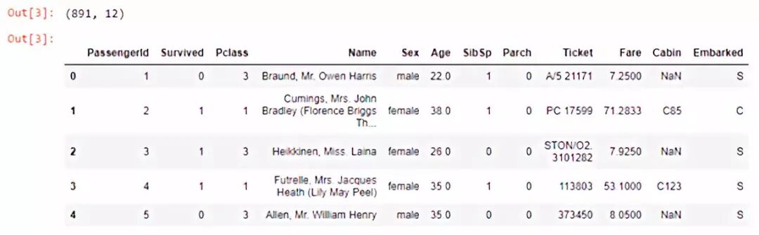
Now that we have loaded the data, we will remove all personally identifiable information. The columns [“PassengerId”, “Name”] contain such information. Note that [“PassengerId”, “Name”] are unique for each row, so they need to be removed later when building machine learning models.
We will also perform similar operations on the columns [“Ticket”, “Cabin”] as these two columns are almost unique for each row.
For demonstration purposes, we will not handle missing values. We will simply ignore all observations that contain missing values.
df.drop(columns=["PassengerId", "Name"], inplace=True) # dropped because unique for every row
df.drop(columns=["Ticket", "Cabin"], inplace=True) # dropped because almost unique for every row
df.dropna(inplace=True)
The result looks like this.
df.shape
df.head()
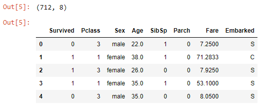
Next, to anonymize more information and as a preprocessing step, we will perform numerical encoding transformations on “Sex” and “Embarked”.
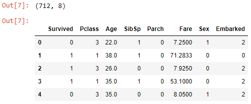
“Sex” will be encoded as “0,1” and “Embarked” will be encoded as “0,1,2”. The LabelEncoder() class does most of the work for us.
encoders = [(["Sex"], LabelEncoder()), (["Embarked"], LabelEncoder())]

mapper = DataFrameMapper(encoders, df_out=True)

new_cols = mapper.fit_transform(df.copy())

df = pd.concat([df.drop(columns=["Sex", "Embarked"]), new_cols], axis="columns")
The DataFrameMapper from the sklearn_pandas package takes a list of tuples as parameters, where the first item of the tuple is the column name and the second item is the transformer.
We are using LabelEncoder() here, but other transformers (e.g., MinMaxScaler(), StandardScaler(), FunctionTransformer()) can also be used.
In the last line, we concatenate the encoded data with the remaining data. Note that you can also write axis = 1, but axis = “columns” is more readable, and I encourage everyone to use the latter.
df.shape
df.head()
df.nunique()
Anonymization by Sampling from the Same Distribution
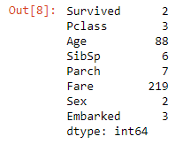
The above code prints the number of unique values for each column. We assume that variables with fewer than 20 unique values are nominal or categorical variables, while those with 20 or more unique values are continuous variables.
We will place the nominal/categorical variables in one list and the other variables in another list.
categorical = []
continuous = []
for c in list(df):
    col = df[c]
    nunique = col.nunique()
    if nunique < 20:
        categorical.append(c)
    else:
        continuous.append(c)
We iterate through all columns with for c in list(df):. For list(df), we could also write df.columns.tolist(), but I prefer list(df).
The core idea of this article is as follows: for each categorical variable, we will calculate the frequency of each value, and then create a discrete probability distribution with the same frequency for each value.
For each continuous variable, we will determine the best continuous distribution from a predefined list of distributions. How do we do this? Once all probability distributions (both discrete and continuous) are determined, we can sample from these distributions to create a new dataset.
Handling Nominal/Categorical Variables
This is a simple example that only requires three lines of code.
for c in categorical:
        counts = df[c].value_counts()
        np.random.choice(list(counts.index), p=(counts/len(df)).values, size=5)
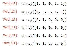
First, we determine the frequency of each unique value in the variable. Then we use this empirical probability function and pass it to np.random.choice() to create a new random variable with the same probability function.
Handling Continuous Variables
Fortunately, there is a discussion on a similar problem on StackOverflow. The main solution is as follows, for each continuous variable:
-
Use a predefined number of bins to create a histogram
-
Try a series of continuous functions to fit the histogram, generating parameters for each function during the fitting process.
-
Find the function with the minimum error (minimum residual sum of squares) that fits the histogram, which will be used to simulate the continuous variable distribution.
The author of this solution neatly divided everything into two functions. I created a third function and placed everything in a file named utils.py, which will be used later in the Jupyter Notebook.
best_distributions = []
for c in continuous:
    data = df[c]
    best_fit_name, best_fit_params = best_fit_distribution(data, 50)
    best_distributions.append((best_fit_name, best_fit_params))
# Result
best_distributions = [
    ('fisk', (11.744665309421649, -66.15529969956657, 94.73575225186589)),
    ('halfcauchy', (-5.537941926133496e-09, 17.86796415175786))]
The best distribution for Age is fisk, and the best distribution for Fare is halfcauchy. Let’s take a look at the results.
plot_result(df, continuous, best_distributions)
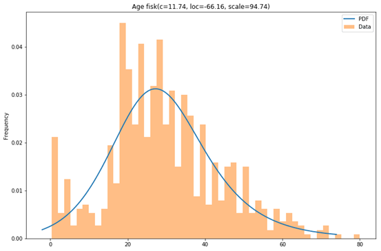
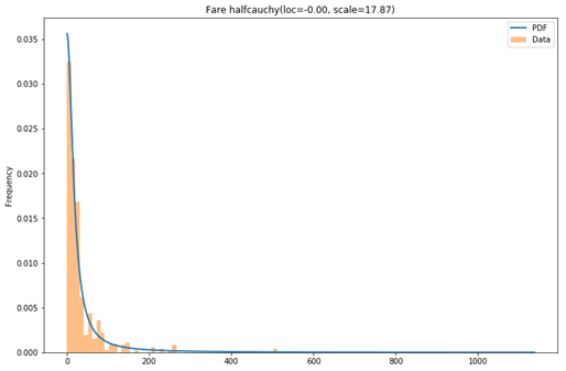
Not bad.
Integrating the Code into a Function
def generate_like_df(df, categorical_cols, continuous_cols, best_distributions, n, seed=0):
    np.random.seed(seed)
    d = {}
    for c in categorical_cols:
        counts = df[c].value_counts()
        d[c] = np.random.choice(list(counts.index), p=(counts/len(df)).values, size=n)
    for c, bd in zip(continuous_cols, best_distributions):
        dist = getattr(scipy.stats, bd[0])
        d[c] = dist.rvs(size=n, *bd[1])
    return pd.DataFrame(d, columns=categorical_cols+continuous_cols)
Now we have a function that can be used to create 100 new observations.
gendf = generate_like_df(df, categorical, continuous, best_distributions, n=100)
gendf.shape
gendf.head()
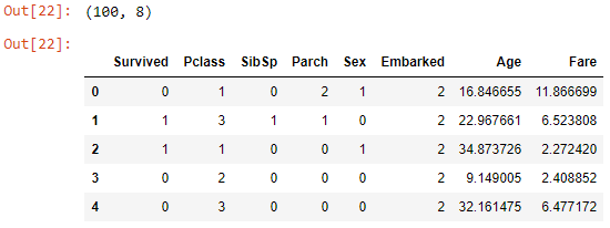
As a post-processing step, we could also anonymize the continuous variables. I chose not to do this. What I did was remove all column names, as they could also leak some information about the dataset, simply replacing them with 0, 1, 2…
gendf.columns = list(range(gendf.shape[1]))
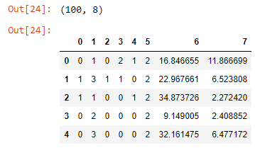
Finally, we are done.
gendf.to_csv("output.csv", index_label="id")
Summary
One drawback of this method is that all interactions between variables are lost. For example, suppose in the original dataset, the chances of survival for females (Sex= 1) are higher (Survived= 1) than for males (Sex= 0), this information is lost in the generated dataset, and any potential relationships between other variables may also be lost.
I hope you find this article useful, and feel free to discuss in the comments section below.
All code in this article
https://github.com/r0f1/dev_to_posts/tree/master/fake_data
Related reports:
https://dev.to/r0f1/a-simple-way-to-anonymize-data-with-python-and-pandas-79g
【Today’s Machine Learning Concept】
Have a Great Definition

Volunteer Introduction
Reply “Volunteer” to join us