Click the blue text above to follow us

📋📋📋 The table of contents is as follows: 🎁🎁🎁
Contents
💥1 Overview
📚2 Results
🎉3 References
🌈4 Matlab Code, Data, Articles


1 Overview
Medium voltage cables have poor signal transmission for high-frequency spectra (such as partial discharge). The propagated signals experience significant attenuation and distortion based on the transmission distance. To understand this process, this paper provides a model to simulate such signals’ transmission in medium voltage cables. Unlike earlier methods, this model does not overlook the waveform characteristics of high-frequency signals. Therefore, an understandable solution to the telegrapher’s equation is provided to describe signal transmission. To use this solution, the propagation constant of the medium voltage cable used must also be known. This propagation constant is calculated based on the individual cable layers, considering all ohmic and dielectric losses. Compared to previous methods, all main line constants are frequency-dependent. The final transmission model can predict the spectrum of the emitted signal at any distance from its origin. Verification results indicate that the predictions and measurements have good accuracy. One potential application of the developed model is to study the transmission of partial discharge on medium voltage cables. This model may also be applicable to high voltage cables. Partial discharge (PD) is a small dielectric breakdown in electrical insulation systems. They can occur locally at any defect point in the insulating material. Unlike a short circuit, the space between two conductors cannot be completely bridged by discharge. Therefore, PD activity can persist for a period and continuously damage the insulation layer. They mainly occur in operating equipment of power transmission systems under high voltage stress. By measuring partial discharge, defects can be detected in time to avoid power outages. Discharges manifest as transient electromagnetic pulses. The pulse width is typically in the nanosecond range. In the frequency domain, this nanosecond pulse consists of a wide spectrum from 0 Hz to several tens of MHz. The shorter the pulse duration, the wider the corresponding spectrum. Most PD’s maximum frequency components should be in the range of 3-100 MHz, corresponding to high frequency (HF) and lower very high frequency (VHF) ranges. When HF signals are mentioned in the following article, it refers to this frequency range. Broadband PD pulses usually must propagate through a transmission line (TL) from their origin to the measuring device, such as overhead lines or power cables. This propagation distorts the initial pulse and reduces the measurable spectrum bandwidth based on the distance traveled. To model and simulate this process, a comprehensive understanding of the propagation behavior of the TL used is necessary. Then, an appropriate model can describe the transmission of PD and all other HF signals on the TL. In this paper, such a model is introduced, where the power line is used as the TL. The investigation uses a medium voltage (MV) cable with a nominal voltage of 20 kV. This cable represents all different voltage levels of medium voltage cables, as their structures are always very similar. Most publications on this signal transmission topic do not consider TL theory, such as [1]-[4]. To correctly simulate the transmission of PD or other HF signals on the TL, a solution to the telegrapher’s equation is required. If the wavelength of the emitted signal is smaller than the length of the TL, these wave equations cannot be neglected. Signals like PD are almost always such. To bridge this research gap, this paper provides a solution to the telegrapher’s equation that describes the transmission of PD along the TL. Similar approaches have been published in [5] and [6]. However, both publications have shortcomings in deriving their solutions. More specifically, both solutions show differences in their right-hand side voltage equations. Additionally, the authors did not provide detailed derivations, making them difficult to understand. These deficiencies are addressed in this work. The quality of signal transmission mainly depends on the medium voltage cable used or its propagation constant. Compared to telecom coaxial cables, power cables are optimized for power transmission at 50 Hz under high voltage conditions. Therefore, the cable structure includes additional semiconductor layers for field control, which have significant attenuation effects, especially on HF signals. To correctly simulate the propagation constant of power cables, these layers must be considered. Despite many publications on this topic, such as [1]-[7], there is still a lack of a purely analytical, comprehensive, and reproducible method to calculate the propagation constant of MV cables. Therefore, this paper aims to provide such a method. The calculation of the propagation constant of the medium voltage cable shown is primarily based on the work of [7]–[9] and combines and extends their results. The frequency dependence of all electrical parameters is considered. Ignoring this frequency dependence is inaccurate for the transmission of HF signals. Detailed explanations can be found in Section 4.


2 Results
%% calculate the voltage and current distribution using the developed transmission model
if locObs>locPD
% right hand side solution
uPropModelF = 1/2.*exp(-gamma.*cableLen).*(exp(gamma.*(cableLen-locObs))+r2.*exp(-gamma.*(cableLen-locObs)))./(1-r1.*r2.*exp(-2*gamma.*cableLen));
iPropModelF = 1/2.*exp(-gamma.*cableLen).*(exp(gamma.*(cableLen-locObs))-r2.*exp(-gamma.*(cableLen-locObs)))./(Zcable.*(1-r1.*r2.*exp(-2*gamma.*cableLen)));
% use the voltage pulse as input source of the transmission model
uPropModelF = uPropModelF.*(exp(gamma.*locPD)-r1.*exp(-gamma.*locPD)).*uGaussF;
iPropModelF = iPropModelF.*(exp(gamma.*locPD)-r1.*exp(-gamma.*locPD)).*uGaussF;
% alternatively use the current pulse as input source
% uPropModelF = uPropModelF.*(exp(gamma.*locPD)+r1.*exp(-gamma.*locPD)).*iGaussF.*Zcable;
% iPropModelF = iPropModelF.*(exp(gamma.*locPD)+r1.*exp(-gamma.*locPD)).*iGaussF.*Zcable;
else
% left hand side solution
uPropModelF = 1/2.*exp(-gamma.*cableLen).*(exp(gamma.*locObs)+r1.*exp(-gamma.*locObs))./(1-r1.*r2.*exp(-2*gamma.*cableLen));
iPropModelF = 1/2.*exp(-gamma.*cableLen).*(-exp(gamma.*locObs)+r1.*exp(-gamma.*locObs))./(Zcable.*(1-r1.*r2.*exp(-2*gamma.*cableLen)));
% use the voltage pulse as input source of the transmission model
uPropModelF = uPropModelF.*(r2.*exp(-gamma.*(cableLen-locPD))-exp(gamma.*(cableLen-locPD))).*uGaussF;
iPropModelF = iPropModelF.*(r2.*exp(-gamma.*(cableLen-locPD))-exp(gamma.*(cableLen-locPD))).*uGaussF;
% alternatively use of the current pulse as input source
% uPropModelF = uPropModelF.*(r2.*exp(-gamma.*(cableLen-locPD))+exp(gamma.*(cableLen-locPD))).*iGaussF.*Zcable;
% iPropModelF = iPropModelF.*(r2.*exp(-gamma.*(cableLen-locPD))+exp(gamma.*(cableLen-locPD))).*iGaussF.*Zcable;
end
%% inverse fourier transform of the resulting voltage signal - alternatively use the resulting current signal
[tPropModel,uPropModelT] = invfourier(f,uPropModelF);
% [~,iPropModelT] = invfourier(f,iPropModelF);
%% example plots
% shifting parameter
width = T*1e09*200;
offset = T*1e09*500; % offset for time domain - pulses should be at zero time
varOffset = T*1e09*max(find(uPropModelT == max(uPropModelT)) - find(uGaussT == max(uGaussT))); % variable offset between model und measured initial pulse
% labels
labelCharge = ['$~' char(string(charge)) '\mathrm{pC}~$'];
labelCableLen = ['$~' char(string(cableLen)) '\mathrm{m}~$'];
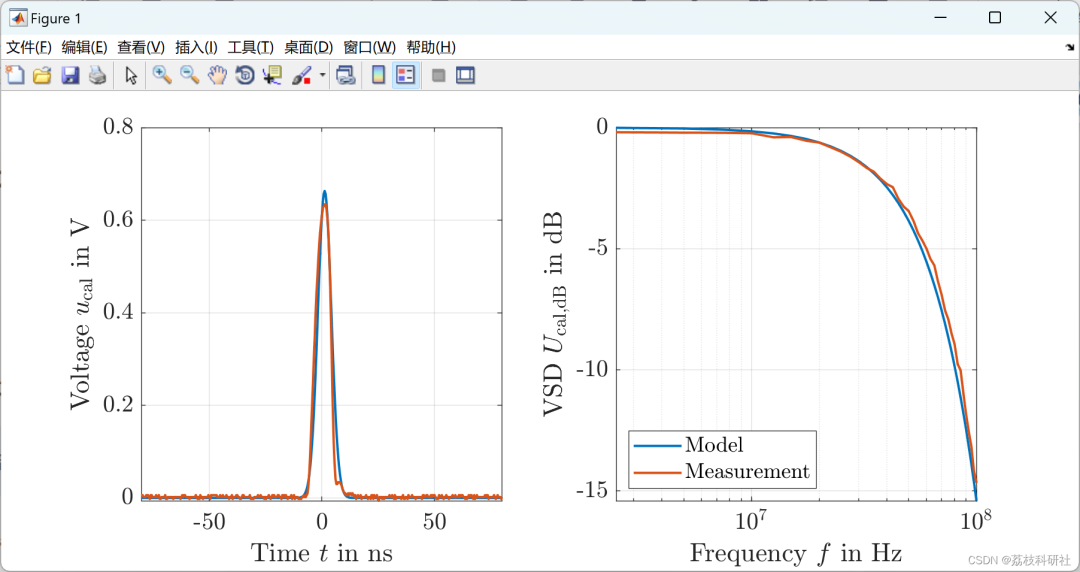
%% plots for comparing measured calibrator pulse and the fitted gaussian model
figure('Color','white','rend','painters','pos',[400250900400])
% time domain comparison
subplot(1,2,1)
plot(t*1e09-offset,uGaussT,t*1e09-offset,uCalMeasT,'LineWidth',1.5)
ylabel('Voltage $u_{\mathrm{cal}}$ in V')
xlim([t(end)*1e09*0.5-width-offset t(end)*1e09*0.5+width-offset])
xlabel('Time $t$ in ns')
set(gca,'FontSize',15)
grid on
% frequency domain comparison - amplitude spectrum
subplot(1,2,2)
semilogx(f,20*log10(abs(uGaussF)/max(abs(uGaussF))),f,20*log10(abs(uCalMeasF)/max(abs(uGaussF))),'LineWidth',1.5)
yline(20*log10(mean(abs(uGaussF(1:5)))/max(abs(uGaussF)))-6,'-',sprintf('$f_{-6dB} =$ %.2f MHz',interp1(20*log10(abs(uGaussF)/max(abs(uGaussF))),f,20*log10(mean(abs(uGaussF(1:5)))/max(abs(uGaussF)))-6)/1e06),'LabelHorizontalAlignment','center','Interpreter','latex','FontSize',14);
ylabel('VSD $U_{\mathrm{cal,dB}}$ in $\mathrm{dB}$')
xlim([0 10e07])
xlabel('Frequency $f$ in Hz')
legend('Model','Measurement','Location','SouthWest')
set(gca,'FontSize',15)
grid on
%sgtitle(['PD calibrator' labelCharge 'input pulse in the time and frequency domain'],'FontSize',15)
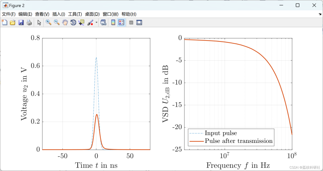
%% comparison of input pulse with the same pulse after one propagation through the cable length
figure('Color','white','rend','painters','pos',[400250900400])
% time domain comparison
subplot(1,2,1)
plot(t*1e09-offset-(t(uGaussT==max(uGaussT))*1e09-offset),uGaussT,'-.')
hold on
plot(tPropModel*1e09-varOffset-offset,uPropModelT,'LineWidth',1.5)
ylabel('Voltage $u_{2}$ in V')
xlim([t(end)*1e09*0.5-width-offset t(end)*1e09*0.5+width-offset])
xlabel('Time $t$ in ns')
set(gca,'FontSize',15)
grid on
% frequency domain comparison - amplitude spectrum
subplot(1,2,2)
semilogx(f(1),20*log10(abs(uGaussF(1))/max(abs(uGaussF)))-6,'-.') % Fake line for correct legend
hold on
semilogx(f,20*log10(abs(uPropModelF)/max(abs(uPropModelF))),'LineWidth',1.5)
%yline(20*log10(mean(abs(uPropModelF(1:5)))/max(abs(uPropModelF)))-6,'-',sprintf('$f_{-6dB} =$ %.2f MHz',interp1(20*log10(abs(uPropModelF)/max(abs(uPropModelF))),f,20*log10(mean(abs(uPropModelF(1:5)))/max(abs(uPropModelF)))-6)/1e06),'LabelHorizontalAlignment','center','Interpreter','latex','FontSize',14);
ylabel('VSD $U_{2, ext{dB}}$ in $\mathrm{dB}$')
xlim([0 10e07])
xlabel('Frequency $f$ in Hz')
legend('Input pulse','Pulse after transmission','Location','SouthWest')
set(gca,'FontSize',15)
grid on
%sgtitle([labelCharge 'pulse after transmission on' labelCableLen 'of cable in the time and frequency domain'],'FontSize',15)

3References
Some theoretical sources are from the internet; please contact us for removal if there is any infringement.

[1] Martin Fritsch (2021) Transmission Model for MV power cables – Mar 3, 2021 10:35


4 Matlab Code, Data, Articles
Public AccountDASHU
Lychee Research Society

MATLAB| Efficiency of Series Coupling Mechanism | Modeling Study of Coupled AntagonismCable Drive Device
2023-11-23
MATLAB| Regional Integrated Energy System Considering Multi-Energy CouplingElectrical Thermal Flow Calculation Study
2024-01-17
MATLAB| Reactive Power Optimization Under the Goal of “Carbon Neutrality”Electrical Interconnected System Active-Reactive Coordination Optimization Model
2023-12-30
MATLAB| Reactive Power Optimization Under the Goal of “Carbon Neutrality”Electrical Interconnected System Active-Reactive Coordination Optimization Model
2023-09-26
MATLAB| Orderly Charging Scheduling Method for Electric Vehicles Considering Different Charging DemandsElectrical Journal Paper Reproduction
2023-06-13
Cold and HeatElectrical Multi-Energy Complementary Micro Energy Network Robust Optimization Scheduling (MATLAB Code Implementation)
2023-04-21

Considering the Uncertainty of New Energy OutputElectrical Equipment Integrated Energy System Collaborative Optimization (MATLAB Code Implementation)
2023-03-12
Cold and HeatElectrical Multi-Energy Complementary Micro Energy Network Robust Optimization Scheduling (MATLAB Code Implementation)
2022-12-14
Multiverse Algorithm Solving Multi-Objective Optimization Problems in Power Systems (MATLAB Implementation) [Electrical Journal Paper Reproduction and Case Innovation]
2022-12-03