Background

In the field of computational advertising, advertisers typically set daily budgets for their promotional plans. The advertising delivery system needs to ensure that the actual daily consumption does not exceed the budget. Additionally, to reach as many users as possible throughout the day, the system usually needs to support Budget Pacing functionality. This feature aims to prevent the budget from being exhausted too early in the first few time slots of the day, instead distributing the budget across various time slots according to a specific mechanism.

The Necessity of Budget Pacing:

Advertiser Perspective:

Early budget consumption (concentrated in the first half of the day) leads to an inability to reach users in the latter half of the day.
Missed potential conversion opportunities affect overall campaign effectiveness.
Budget pacing helps reach a more diverse user group.

Advertising Platform Perspective:

Intense competition in the first half of the day and reduced competition in the latter half can lead to decreased potential revenue for the platform due to the second-price auction mechanism (the more intense the competition, the better the platform’s revenue potential).
Budget pacing can maintain a high level of competition throughout the day, improving average ECPM.
It stabilizes system load, avoiding peak traffic pressure.
Provides advertisers with better options for campaign effectiveness.

Implementation Ideas for Budget Pacing

There are mainly two approaches:

Probabilistic Throttling:

Traffic Prediction: Based on the granularity of the advertising plan, predict its exposure throughout the day and in each time slot; simultaneously predict overall traffic.
Budget Allocation Plan: Calculate the budget allocation ratio for each time slot based on traffic predictions.
Adjusting the Win Rate: During the advertising delivery process, monitor budget consumption in real-time and dynamically adjust the bid rate (win rate) corresponding to the advertising plan.

Bid Modification:

Control the speed of budget consumption by dynamically adjusting the advertising bid. The higher the bid, the greater the probability of winning exposure, and correspondingly, the higher the advertising consumption.

Ultimate Goal: Based on accurate predictions of the daily visitation patterns of the target audience, concentrate budget consumption on the most relevant Top-N users to achieve optimal delivery results.

Solution: Application of PID Controller

The PID controller is a classic algorithm in the field of automatic control, widely used in industrial control. Its core lies in introducing a feedback mechanism: the deviation between the actual value of the controlled variable (such as consumption) and the expected value serves as the input signal, which the controller uses to adjust the control variable (such as bid), and then the actuator (such as the bidding system) applies the influence, ultimately bringing the actual value of the controlled variable closer to the expected value.

Thus, we can treat advertising bid as the control variable and consumption as the controlled variable. Based on the deviation between the actual and expected consumption values for each time slot, dynamically adjust the bid for the next time slot to make the actual consumption approach the expected value:

If the actual consumption is below the expected value -> increase the bid -> win more exposure in the next time slot -> increase consumption.
If the actual consumption is above the expected value -> decrease the bid -> win less exposure in the next time slot -> reduce consumption.

Interpretation of PID Components (Taking Consumption Rate as an Example)

Proportional (P) Component: Reflects the instantaneous deviation between the expected consumption rate and the actual consumption rate for the current time slot (e(n) = r(n) - c(n)).
Integral (I) Component: Reflects the accumulation (integral) of historical consumption rate errors, i.e., cumulative spending error (Σe(n)), eliminating steady-state error.
Derivative (D) Component: Reflects the trend of consumption rate error (de(n)/dt ≈ e(n) - e(n-1)), providing anticipatory adjustment.

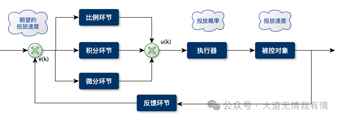
Real-Time Budget Pacing for DSP Advertising Based on PID Controller — WX20241031-223007@2x

Design of the Bid Controller

u(n): Advertising bid (updated at the end of time slot n for use in time slot n+1).
r(n): Expected consumption for time slot n.
c(n): Actual consumption for time slot n.
e(n) = r(n) - c(n): Consumption deviation for time slot n.

At the end of time slot n and the beginning of time slot n+1, the current bid adjustment amount Δu is calculated based on the following incremental PID formula:

$\Delta u = (k_p+k_i+k_d)e(n) – (k_p+2k_d)e(n-1)+ k_de(n-2)$

Update the bid based on Δu for the next time slot:$u(n) = u(n-1)+\Delta u$

Finally, constrain the bid within upper and lower limits:

$u(n)=\begin{cases} u_{min} & u(n)<= u_{min} \\ u(n) & u_{min} < u(n) <= u_{max} \\ u_{max} & u(n) >= u_{max} \end{cases}$

Incremental PID Controller Code Example:

class Incr_PID_Controller:
    def __init__(self, k_p, k_i, k_d, bid, ratio):
        self.k_p = k_p  # Proportional coefficient
        self.k_i = k_i  # Integral coefficient
        self.k_d = k_d  # Derivative coefficient
        self.bid = float(bid)  # Current bid
        self.raw_bid = float(bid)  # Original initial bid
        self.e = 0  # Current deviation e(n)
        self.e_1 = 0  # Previous time slot deviation e(n-1)
        self.e_2 = 0  # Two time slots ago deviation e(n-2)
        self.max_bid = bid * (1 + ratio)  # Bid upper limit
        self.min_bid = bid * (1 - ratio)  # Bid lower limit
        self.ratio = ratio  # Maximum adjustment ratio

    def update(self, budget, spent):
        """Update bid based on budget and actual consumption"""
        if budget &lt;= 0:  # Avoid division by zero
            return
        # Update historical deviations: e(n-2) &lt;- e(n-1), e(n-1) &lt;- e(n)
        self.e_2 = self.e_1
        self.e_1 = self.e
        # Calculate current deviation e(n) = expected consumption(r(n)) - actual consumption(c(n))
        self.e = budget - spent
        # Calculate increment Δu (PID formula)
        diff = ((self.k_p + self.k_i + self.k_d) * self.e
                - (self.k_p + 2 * self.k_d) * self.e_1
                + self.k_d * self.e_2)

        # Calculate Δu relative to budget (normalized)
        r = float(diff) / budget
        # Convert ratio r to bid adjustment amount (based on original bid and allowed adjustment ratio)
        price = self.bid * self.ratio * r
        # Apply adjustment and constrain within [min_bid, max_bid]
        self.bid = round(max(self.min_bid, min(self.bid + price, self.max_bid)))

    def init_data(self, budget, spent):
        """Initialize or reset controller state (e.g., at the start of a new day)"""
        if abs(budget - spent) &gt; self.raw_bid:
            self.update(budget, spent)  # Use large deviation to trigger an update to initialize bid
        else:
            self.bid = self.raw_bid  # Otherwise reset to original bid
        self.e = 0  # Reset deviation records
        self.e_1 = 0
        self.e_2 = 0

    def get_bid(self):
        """Get current bid"""
        return self.bid

Advertising Environment Simulation

The real advertising bidding environment involves multi-party games and dynamic changes, making it difficult to accurately model the deterministic relationship between bid u and actual consumption c. To simplify the simulation, we use the following function to describe this relationship:

$c=0.124 * u^2 + 0.876* u + \epsilon$

Where:

u: Time slot bid (float, range 1 to 100).
c: Actual consumption for the time slot.
ε: Noise term, following a standard normal distribution N(0, 1).

This function ensures that c monotonically increases with u:

u = 1 -> c ≈ 1 + ε.
u = 100 -> c ≈ 1327.6 + ε.
Thus, c is roughly between 1 and 1328.

def ad_env(u):
    """Simulate advertising environment: input bid u, return actual consumption c"""
    return 0.124 * pow(u, 2) + 0.876 * u + np.random.normal(0, 1, 1)[0]

Simulation of Budget Pacing Effects

Initialize PID controller: Kp=0.01, Ki=0.02, Kd=0.01, initial bid u=70. Simulate a day with 96 time slots (one slot every 15 minutes), with the expected consumption r(n) calculated from a bimodal traffic distribution (two overlapping normal distributions), with a total daily budget of 1000 yuan.

if __name__ == '__main__':
    # Time slots: 0 to 95, a total of 96 time slots
    t = np.arange(0, 96, 1)
    # Calculate expected consumption for each time slot (bimodal traffic distribution)
    r = 100000 * (0.5 * norm.pdf(t, loc=20, scale=15) + 0.5 * norm.pdf(t, loc=70, scale=15))
    # Initialize PID controller
    pid_controller = Incr_PID_Controller(0.01, 0.02, 0.01, 70)

    c = []  # Store actual consumption
    for n in t:
        u = pid_controller.get_bid()  # Get current bid
        c_n = ad_env(u)  # Simulate delivery, get actual consumption
        c.append(c_n)
        # Update controller based on expected consumption r[n] and actual consumption c_n for time slot n, get bid for time slot n+1
        pid_controller.update(r[n], c_n)
        u_next = pid_controller.get_bid()  # Get updated bid (for next time slot)
        print(
            'Time slot [{:02d}], Bid: {:.2f}, Actual Consumption: {:.2f}, Expected Consumption: {:.2f}, Updated Bid: {:.2f}, Adjustment: {:.2f}'.format(
                n, u, c_n, r[n], u_next, u_next - u))

    # Plot expected consumption (r, red) and actual consumption (c, blue) curves
    plt.plot(t, r, linewidth=3, color='r', marker='o', markerfacecolor='blue', markersize=4)
    plt.plot(t, c, linewidth=3, color='b', marker='o', markerfacecolor='red', markersize=4)
    plt.show()

Summary of Simulation Output (First and Last Few Time Slots):

“

In time slot [00], Bid: 70.00, Actual Consumption: 667.60, Expected Consumption: 546.73, Updated Bid: 65.16, Adjustment: -4.84 In time slot [01], Bid: 65.16, Actual Consumption: 583.05, Expected Consumption: 596.23, Updated Bid: 69.32, Adjustment: 4.15 … In time slot [94], Bid: 59.97, Actual Consumption: 499.03, Expected Consumption: 369.74, Updated Bid: 57.43, Adjustment: -2.53 In time slot [95], Bid: 57.43, Actual Consumption: 458.82, Expected Consumption: 331.60, Updated Bid: 54.91, Adjustment: -2.52

Effect Visualization:

Red Curve: Expected consumption for each time slot r(n).
Blue Curve: Actual consumption for each time slot c(n).

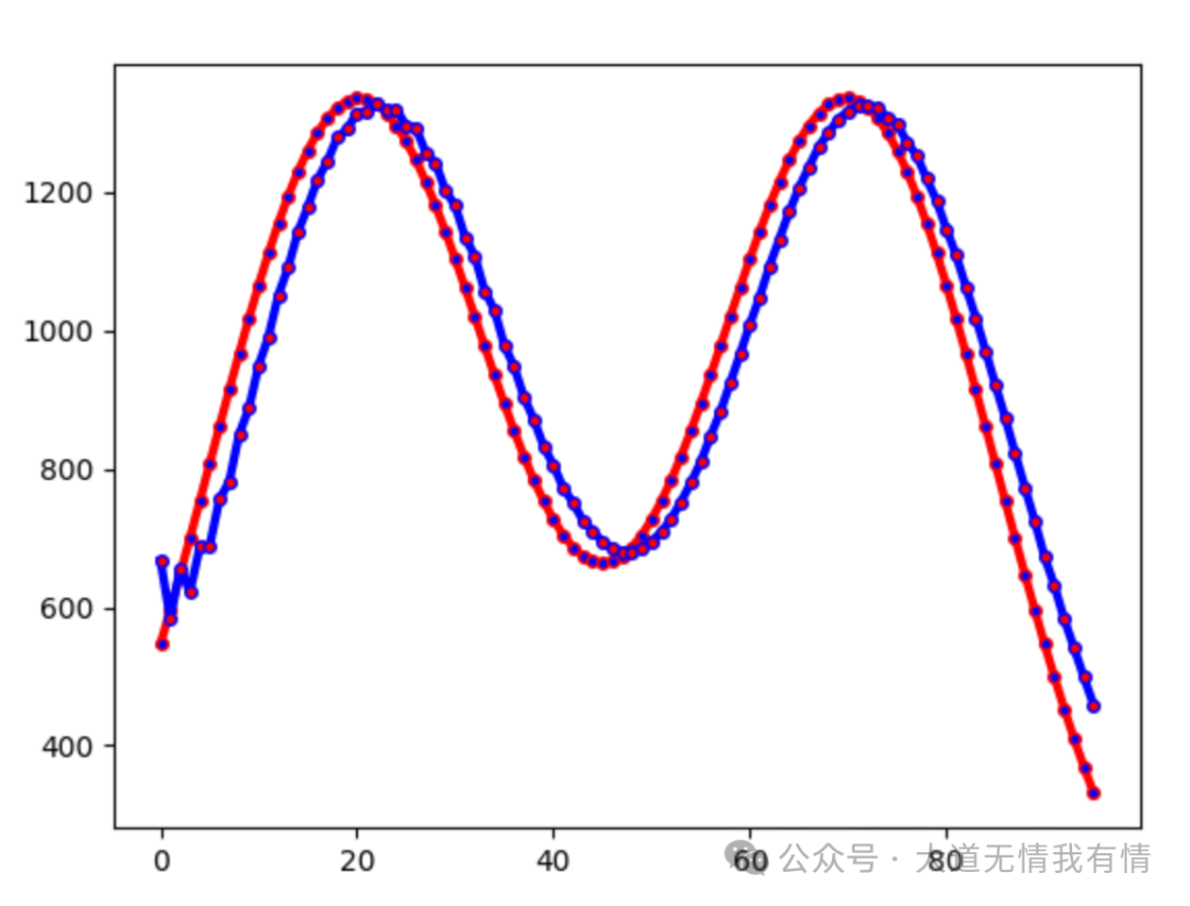
Conclusion: Except for the initial time slot where the system startup causes fluctuations, the actual consumption values c(n) closely follow the expected consumption values r(n), effectively achieving the goal of budget pacing.

Key Points and Practical Experience

The theoretical model is clear, but practical application needs to address many issues, mainly involving data processing and pricing strategies:

Data Aspects

Real-Time Data is Fundamental: Obtaining real-time click, conversion, and consumption data is crucial. Data delays can significantly weaken the effectiveness of PID control.
Account and Plan Status: Accurate acquisition of current account balance, current plan balance, current plan budget, plan delivery time slots, and plan start-stop status is necessary.
Task Reliability: Near-line tasks need to consider the possibility of update failures. Recording whether each bid update is successful is key to troubleshooting and ensuring system robustness.
Initial Bid Setting:

For Historical Plans: Use a certain percentage of recent actual costs as the initial bid.
For New Plans: Reference bids from similar industry and conversion type plans.

Data Alignment: Before each round of calculations, budget and consumption data need to be formatted based on bid update status, plan delivery status, etc., to ensure data is correctly associated with its corresponding bid effective time slot.

Strategy Aspects

Normalize Inputs: Directly using the absolute deviation of budget-consumption (e(n)) is not conducive to PID parameter tuning (as different plans have significant scale differences). It is recommended to use the budget completion rate (actual consumption / expected consumption) as normalized input, which is more stable and easier to tune.
Control Bid Adjustment Magnitude: Limit each bid adjustment to a fixed percentage of the last bid (e.g., ±20%). This avoids drastic bid fluctuations due to data delays or noise, preventing budget overspending or cost surges.
Rapid Suppression Mechanism: When consumption is detected to far exceed the budget (e.g., completion rate > 150%), and conventional PID adjustments may be too slow, trigger a rapid discount strategy (e.g., directly halving the current bid) to quickly curb overspending.
I-term Adjustment (Practical Optimization): The initial PID version used single time slot errors. In practice, it was adjusted to calculate errors based on cumulative budget and consumption (Σ(expected consumption - actual consumption) / total budget), which better reflects overall budget execution deviation and yields better results.
D-term Trade-off: In our application, we only used the P and I terms. The role of the derivative term (D) overlaps with the constraints on the magnitude of bid changes between control periods (see strategy point 2).
End-of-Day Processing: At the end of the last time slot of the day, significantly reduce the bid (e.g., to the minimum value) to prevent overspending at the start of the next day due to state synchronization delays and other issues.

Engineering Architecture

PID Pricing Trigger Timing:

Scheduled Tasks: Trigger calculations at fixed time intervals (e.g., every 15 minutes).
Consumption Event Trigger: Trigger when advertising budget is consumed. Typically, this adjustment will be more conservative than the last (due to increased consumption), helping to improve the winning probability of other ads.

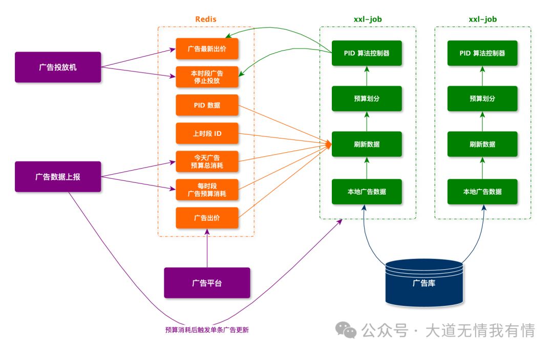
System Process Overview:

XXL-Job: Periodically execute PID calculation tasks, pushing the latest bid and advertising delivery status to Redis.
Ad Filtering and Bidding: When advertising opportunities arise, the filtering service retrieves ad status and the latest bid from Redis, filtering out non-deliverable ads and using the latest bid to participate in bidding.
Winning Report Triggers Bid Adjustment: Winning messages can trigger PID bid adjustments for individual ads (supplementing the gaps in scheduled tasks).
Status Sharing: Since XXL-Job executes across multiple machines, intermediate states of PID calculations (such as e, e_1, e_2, bid) need to be stored in Redis for use in subsequent calculations by other instances.
Data Timeliness: Before each bid adjustment calculation, the latest bid, daily budget, and actual consumption data must be retrieved from Redis to ensure calculations are based on the latest state.

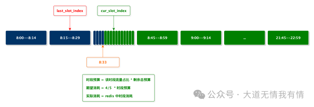
Budget Allocation Timing:

New Ads Joining: Initialize their budget allocation across time slots.
Time Slot Transition: Transitioning from time slot n to n+1 is a critical point for reallocating budgets. At this time, consider any overspending or underspending that may have occurred in the previous time slot and adjust the budget allocation for subsequent time slots.

Time Slot Division and Budget Allocation:

Divide time slots into every 15 minutes, totaling 96 time slots in a day.
Need to count historical traffic distribution in each time slot.
Allocate budgets for each time slot based on historical traffic distribution ratios.

Summary and Expansion

The above solution is based on the Bid Modification approach, utilizing an incremental PID controller to regulate bids for budget pacing. This controller is also applicable to the Probabilistic Throttling approach, requiring only changes to the control variable and regulation logic:

Only need to satisfy budget constraints: The control variable u(n) can be the bid rate. If overspending occurs, decrease u(n), and if underspending occurs, increase u(n).
Budget Constraints + Click Maximization: The control variable u(n) can be the estimated click-through rate threshold. If overspending occurs, increase u(n) (filtering low CTR traffic), and if underspending occurs, decrease u(n) (relaxing traffic restrictions).

The examples provided demonstrate the application of PID under ideal conditions. In real advertising scenarios, it is necessary to combine practical guidelines such as “Using PID for Budget Control” to deeply address the data and strategy details mentioned in the “Key Points” (such as real-time data construction, initialization strategies, normalization processing, safety constraints, etc.).

Universality of PID Controllers: PID controllers are widely applied in computational advertising. Their core value lies in the ability to effectively regulate when the control variables (such as bids, bid rates, thresholds) and controlled variables (such as consumption, costs, business metrics) cannot be precisely modeled in a feedforward manner.

Other Application Scenario Examples:

Cost Assurance (oCPX):

Controlled Variable: Actual conversion cost.
Control Variable: Billing discount coefficient.
Regulation Logic: If actual cost > target cost -> lower the discount coefficient (less billing); if actual cost < target cost -> raise the discount coefficient (more billing). This brings actual costs closer to the target.

Automatic Bidding:

Regulate bids to make final ROI, CPA, and other business metrics approach the target values set by advertisers. The paper “Bid Optimization by Multivariable Control in Display Advertising” elaborates on an automatic bidding scheme based on multivariable feedback control.

PID controllers, as a powerful feedback control tool, provide an effective and engineerable approach to solving dynamic optimization problems in online advertising systems.