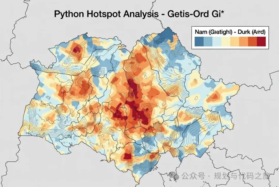
Python Hotspot Analysis: Identifying Statistically Significant Spatial Clusters

Using spatial statistics to distinguish meaningful patterns from random noise.

Spatial data often exhibits clustering phenomena. Crimes concentrate in specific neighborhoods, disease cases cluster in certain areas, heat forms hotspots, economic activities tend to aggregate, and traffic accidents concentrate at certain intersections. These clusters may represent meaningful patterns that require attention, but they may also just be fluctuations in random data.

Visual inspection alone cannot distinguish statistically significant clusters from random spatial variation. Human pattern recognition abilities can “see” clusters even in purely random data. A few crime incidents occurring in a certain area may appear as a “hotspot,” but it could merely be coincidental. Without statistical testing, superficial patterns can mislead analysis and decision-making.

Hotspot analysis applies spatial statistical methods to identify clusters that are unlikely to be produced by random chance. It answers a key question: “Is the observed spatial concentration statistically significant, or could it be caused by random processes?” This distinction separates true patterns that require action from false patterns that waste resources.

Python, through its spatial statistics libraries, provides comprehensive tools for rigorous hotspot analysis. Public health analysts use it to identify disease outbreak areas, law enforcement uses it to target crime prevention efforts, urban planners use it to locate service gaps, environmental scientists use it to detect pollution sources, and emergency managers use it to identify risk areas. All of these rely on statistically validated hotspot analysis.

Understanding hotspot analysis methods, their assumptions, and appropriate applications helps in reliable spatial pattern recognition, thereby supporting evidence-based decision-making.

Below is a comprehensive guide to performing hotspot analysis using Python.

🗺️ Understanding Spatial Clustering

Before applying statistical tests, understanding the concept of clustering helps clarify what hotspot analysis reveals.

Spatial Autocorrelation measures whether values at neighboring locations are similar.

Tobler’s First Law of Geography—”Everything is related to everything else, but near things are more related than distant things”—describes positive spatial autocorrelation as a fundamental principle of geography.

Positive Autocorrelation means similar values cluster together (high values next to high values, low values next to low values).
Negative Autocorrelation means dissimilar values are adjacent (high values next to low values).
Zero Autocorrelation means spatial independence, where values are unrelated to their neighbors.

Point Pattern Clustering describes the non-uniform distribution of point locations.

Complete Spatial Randomness (CSR) refers to points being uniformly randomly distributed in space.
Clustered Pattern indicates points are concentrated in certain areas.
Regular Pattern indicates points are evenly spaced.

Local Clustering vs. Global Clustering: Global statistics (e.g., Moran’s I) measure whether clustering exists overall in the data; local statistics (e.g., Local Moran’s I, Getis-Ord Gi*) identify specific locations where clustering occurs.

Global statistics answer: “Is there clustering?”
Local statistics answer: “Where is the clustering?”

Hotspots vs. Coldspots: Hotspots are clusters of high values (e.g., high crime rates); Coldspots are clusters of low values (e.g., low income levels, i.e., affluent hotspots).
Statistical Significance: Distinguishing observed clustering from random chance. Significant clustering is unlikely to occur randomly, suggesting meaningful processes.

📈 Global Clustering Measures

Global statistics quantify the overall spatial autocorrelation of the entire study area.

Moran’s I: The most commonly used global autocorrelation statistic. It measures whether values at nearby locations are more similar than expected under spatial randomness.

Ranges from -1 (complete dispersion) to 0 (random) to +1 (complete clustering).
Determined through a permutation test to see if the observed Moran’s I is significantly different from zero.

Geary’s C: Another global autocorrelation measure. It focuses more on variance rather than covariance, making it more sensitive to local differences.

Ranges from 0 (positive autocorrelation) to 1 (no autocorrelation) to 2+ (negative autocorrelation).

Getis-Ord General G: Measures the overall concentration of high or low values. A high G value indicates high values cluster together, specifically used for detecting hotspot/coldspot patterns.

The limitations of global statistics are that they only provide a single summary of the area and cannot reveal where clustering occurs, nor can they distinguish between hotspots and coldspots. They need to be used in conjunction with local statistics.

📍 Local Indicators of Spatial Association (LISA)

Local statistics identify specific locations contributing to clustering.

Local Moran’s I: Decomposes global Moran’s I into contributions from each location. It identifies four types of clusters:

High-High: High values surrounded by high values (hotspot).
Low-Low: Low values surrounded by low values (coldspot).
High-Low: High values surrounded by low values (spatial outlier).
Low-High: Low values surrounded by high values (spatial outlier).
Mapping significant High-High clusters reveals hotspots.

Getis-Ord Gi and Gi* statistics: Specifically used to identify statistically significant **high values (hotspots)** or **low values (coldspots)** spatial clustering.

Gi statistic: Compares the sum of values within a neighborhood to the sum of values across the entire study area (excluding the location itself).
Gi* statistic: Includes the location itself in the neighborhood sum.
A high positive Z score indicates a hotspot; a high negative Z score indicates a coldspot.

Choosing between Local Moran’s I and Getis-Ord:

Characteristic	Local Moran’s I	Getis-Ord Gi / Gi*
Type of Identification	Outliers and clusters (four types)	Specifically for hotspots/coldspots (high-low concentration)
Benchmark	Based on deviation from the mean	Based on absolute values
Application Preference	Comprehensive understanding of spatial relationships	Targeting high-value concentrations (e.g., crime, disease)

Running both statistics often provides the most complete understanding.

🔗 Defining Spatial Relationships

Spatial statistics require defining relationships between locations—what constitutes neighbors and the strength of interactions between them. This is achieved through a spatial weight matrix (W).

Contiguity-based weights: Suitable for polygonal data (e.g., administrative boundaries), defining neighbors based on whether units are adjacent (e.g., Queen adjacency or Rook adjacency).
Distance-based weights: Suitable for point data or situations where influence extends beyond immediate neighbors.

Fixed distance bands: Include all units within a threshold distance.
K-nearest neighbors (KNN): Include the K closest units.
Inverse distance weights: Weights are inversely proportional to distance (closer units have more influence).

Network-based weights: Suitable for phenomena constrained by networks (e.g., roads, rivers).
Weight normalization: Row-standardization (where the sum of weights per row equals 1) is typically preferred, as it prevents bias due to varying numbers of neighbors.

Key Point: The results of hotspot analysis are sensitive to the definition of spatial weights. Best practice is to test sensitivity; patterns that appear under multiple weight definitions are more reliable.

📊 Multiple Testing Correction

Conducting statistical tests at many locations raises the multiple comparison problem.

Multiple Comparison Inflation: At a significance level of $\alpha = 0.05$, even without clustering, 5% of tests will incorrectly reject the null hypothesis (false positives). Testing hundreds or thousands of locations greatly exaggerates the risk of false positives.
Bonferroni Correction: Adjusts the significance level $\alpha$ by dividing it by the number of tests $n$ (i.e., $\alpha/n$). It is too conservative and often misses true hotspots.
False Discovery Rate (FDR) Control: Controls the proportion of false positives among the conclusions deemed discoveries.

Benjamini-Hochberg procedure provides FDR control, being less conservative than Bonferroni, allowing for the identification of more true hotspots while keeping false discoveries within an acceptable proportion.

Due to the presence of spatial autocorrelation, standard multiple testing corrections (which assume independence) may not be precise enough. In practice, FDR correction is often combined with a requirement for spatial consistency (isolated significant locations may be false positives).

💻 Implementation with Python and PySAL

PySAL (Python Spatial Analysis Library) provides comprehensive spatial statistical functionality.

Installation and Setup: Install via pip install pysal or its modular components (libpysal, esda, splot).
Creating Spatial Weights (libpysal.weights):

Create adjacency weights from GeoDataFrame (Queen/Rook).
Create distance weights (distance bands, K-nearest neighbors, kernel weights).

Global Autocorrelation (esda):

Moran, Geary, G functions for calculating statistics and conducting significance tests via permutation.

Local Statistics (esda):

Moran_Local for local Moran’s I and clustering classification.
G_Local and Getis_Ord for Getis-Ord Gi / Gi*.

Visualization (splot):

Moran scatter plots.
LISA cluster maps (distinguishing four types).
Getis-Ord hotspot maps (showing significant hotspots and coldspots).

Workflow: Typically: Load data $\rightarrow$ Create weight matrix $\rightarrow$ Calculate global statistics $\rightarrow$ Calculate local statistics $\rightarrow$ Apply corrections $\rightarrow$Map and interpret.

PySAL makes complex spatial statistics easily accessible in the Python environment.

💡 Scan Statistics and Moving Windows

Scan Statistics systematically search for clusters without pre-specifying locations.

Spatial Scan Statistic: Moves a circular or elliptical window across the study area, testing whether clustering within each window is significant. It identifies most likely clusters and secondary clusters.
Likelihood Ratio Test: Compares the observed number of cases within the window to the expected number of cases under the null hypothesis.
SaTScan Software: Widely used in epidemiology for implementing spatial, temporal, and spatiotemporal scan statistics.

Advantages: No need to pre-specify potential cluster locations, systematically searching across different scales and locations, with rigorous statistical testing via permutation.

Scan statistics are primarily applied in disease outbreak detection, complementing local spatial statistics.

🕰️ Spatiotemporal Hotspot Analysis

Clustering often changes over time, necessitating spatiotemporal analysis methods.

Types of Hotspots:

Emerging Hotspots: Recently formed clusters.
Persistent Hotspots: Areas that maintain clustering over time (chronic issues).
Intermittent Hotspots: Clusters that alternate between clustering and non-clustering.
Oscillating Hotspots: Alternating between hot and cold patterns.

Space-time Cube: Organizes data with spatial dimensions as the base and time as the third dimension.
Getis-Ord Gi with time*: Calculates hotspot statistics at multiple time points, tracking how hotspots emerge, persist, or dissipate.
Spatiotemporal Interaction Tests: Determine whether clustering is purely spatial, purely temporal, or a true spatiotemporal interaction.

Spatiotemporal analysis reveals dynamics—how patterns change over time, rather than just static spatial patterns at a single time point.

🌐 Cross-Disciplinary Applications and Interpretations

Hotspot analysis serves various fields and has field-specific considerations.

Field	Application Example	Key Considerations
Public Health	Disease clusters, cancer clustering, resource allocation	Ethical considerations (avoiding stigmatization), ensuring health equity.
Crime Analysis	Crime concentration, police deployment, prevention programs	Statistical rigor (preventing biased policing), community interventions.
Traffic Safety	Accident hotspots, road improvements, safety campaigns	Avoid wasting resources on random clusters.
Economic Geography	Industry clustering, poverty concentration, opportunity distribution	Analysis of spatial inequality patterns.
Ecology	Species concentration areas, biodiversity hotspots	Prioritize protection of statistically significant concentration areas.

Interpretation and Communication:

Distinguish between statistical significance and practical significance (effect size).
The confidence in identified hotspots depends on: statistical significance (low p-values), effect size (large z-scores), consistency across methods, and support from domain knowledge.
Mapping Standards: Use diverging color schemes (red-hot, blue-cold), only display statistically significant clusters, and provide context.
Narrative Explanation: Translate statistical data into understandable language and actionable recommendations (e.g., “The crime rate in this community is three times higher than surrounding areas”).

⚠️ Limitations and Considerations

Hotspot analysis is not without limitations.

Modifiable Areal Unit Problem (MAUP): Results depend on how spatial units are aggregated (e.g., different administrative boundaries or grid sizes). The robustness of patterns should be tested across different scales.
Edge Effects: Locations near the boundaries of the study area may lead to statistical bias due to incomplete neighborhoods.
Data Quality: Reporting bias, measurement errors, or missing data can affect analysis.
Ecological Fallacy: Cannot infer individual-level relationships from aggregate-level patterns (e.g., a crime hotspot does not mean all residents in that area are criminals).
Spatial Scale Effects: The appropriate scale of analysis depends on the process being studied.
Temporal Instability: Patterns may change over time, requiring regular updates to analysis.

✅ Best Practices and Recommendations

Following established principles can lead to effective hotspot analysis.

Start with Exploratory Visualization: Reveal surface patterns through maps before formal testing.
Select Appropriate Methods: Use point pattern methods for point data, LISA or Getis-Ord for polygon data.
Carefully Define Spatial Relationships: Create weight matrices that reflect spatial processes and test their sensitivity.
Apply Multiple Testing Corrections: Control for false discoveries.
Validate Results: Compare with alternative data sources or replicate over time.
Combine Global and Local Statistics: Obtain a complete picture.
Consider Temporal Dynamics: Distinguish between emerging and persistent issues.
Integrate Domain Knowledge: Use disciplinary context to interpret statistical results.
Thoroughly Document Methods: Include data sources, weights, thresholds, and corrections.
Communicate Clearly: Translate statistical analysis into practical value and actionable insights.

Hotspot analysis transforms superficial visual patterns into statistically validated clusters, distinguishing signal from noise in spatial data. Rigorous spatial statistics can confidently identify meaningful spatial concentrations that require attention while avoiding false alarms from random variations.