Peridogram
This function can implement the periodogram and improved periodogram method. The basic syntax is to use the default rectangular window and DFT length to obtain the periodogram. The DFT length is the next power of 2 greater than the signal length. Since the signal is real-valued and of even length, the periodogram is one-sided with one point. The output is the normalized power spectral density.
Perform non-normalization processing::: hljs-center
:::
Using the Hamming window and the default DFT length to obtain the modified periodogram. The DFT length is the next power of 2 greater than the signal length. Since the signal is real-valued and of even length, the periodogram is one-sided with one point.
Using the Hamming window to correct the periodogram
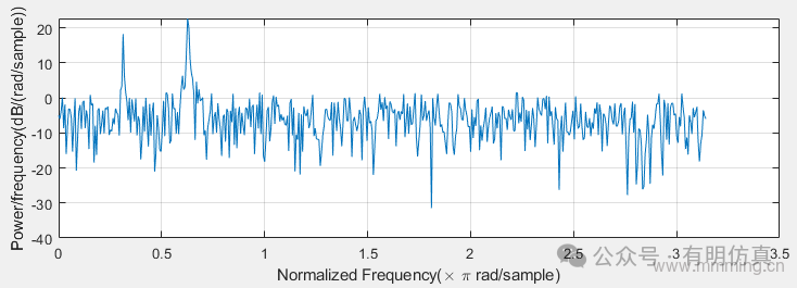
Create a sine wave with angular frequency π/4 rad/sample plus N(0,1) white noise. The signal length is 320 samples. Use the default rectangular window and a DFT length equal to the signal length to obtain the periodogram. Since the signal is real-valued, the one-sided periodogram returned by default has a length equal to 320/2+1.
n = 0:319;
x = cos(pi/4*n)+randn(size(n));
nfft = length(x);
periodogram(x,[],nfft)
::: hljs-center
:::
Return the two-sided periodogram estimate at the specified normalized frequencies in the vector. w must contain at least two elements; otherwise, the function will interpret it as nfft.
n = 0:319;
x = cos(pi/4*n)+0.5*sin(pi/2*n)+randn(size(n));

[pxx,w] = periodogram(x,[],[pi/4 pi/2]);
pxx

>>pxx = 1×2

   14.0589    2.8872
n = 0:319;
x = cos(pi/4*n)+0.5*sin(pi/2*n)+randn(size(n));
[pxx1,w1] = periodogram(x);
plot(w1/pi,pxx1,w/pi,2*pxx,'o')
legend('pxx1','2 * pxx')
xlabel('\omega / \pi')::: hljs-center
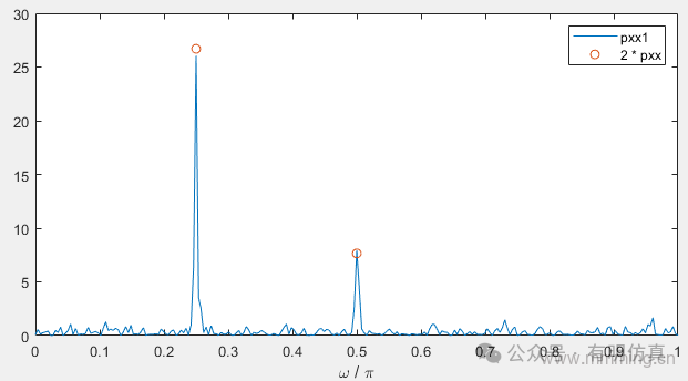
::: The obtained periodogram values are half of the one-sided periodogram values. When evaluating the periodogram at a specific set of frequencies, the output is a two-sided estimate.
Return the two-sided periodogram estimate at the specified frequencies in the vector. The vector f must contain at least two elements; otherwise, the function will interpret it as nfft. The frequency f is the number of cycles per unit time.
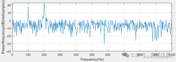
Create a signal consisting of two sine waves at 100 and 200 Hz plus N(0,1) white noise. The sampling frequency is 1 kHz. Obtain the two-sided periodogram at 100 and 200 Hz.
t = 0:0.001:1-0.001;
x = cos(2*pi*100*t)+sin(2*pi*200*t)+randn(size(t));

freq = [100 200];
pxx = periodogram(x,[],freq,fs)

>>pxx = 1×2

    0.2647    0.2313
Return the 100% confidence interval for the PSD estimates in the probability vector pxxc. The following example illustrates the use of confidence intervals with the periodogram. Although it is not a necessary condition for statistical significance, frequencies where the confidence lower limit in the periodogram exceeds the confidence upper limit of the PSD estimate clearly indicate significant oscillations in the time series.
Create a composite white noise signal N(0,1) with 100 Hz and 150 Hz sine waves added. The amplitudes of the two sine waves are 1. The sampling frequency is 1 kHz.
fs = 1000;
t = 0:1/fs:1-1/fs;
x = cos(2*pi*100*t) + sin(2*pi*150*t) + randn(size(t));
[pxx,f,pxxc] = periodogram(x,rectwin(length(x)),length(x),fs,...
    'ConfidenceLevel',0.95);

plot(f,10*log10(pxx))
hold on
plot(f,10*log10(pxxc),'-.')

xlim([85 175])
xlabel('Hz')
ylabel('dB/Hz')
title('Periodogram with 95%-Confidence Bounds')
Obtain the periodogram PSD estimate with 95% confidence limits. Plot the periodogram and confidence intervals, zooming in on the target frequency region around 100 and 150 Hz. ::: hljs-center
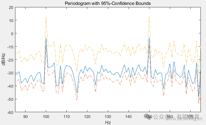
:::
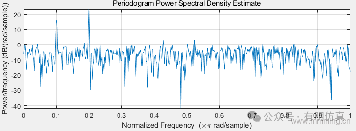
Reassign each PSD estimate to the frequency closest to its energy center. rpxx contains the sum of estimates assigned to each element of f. Obtain a periodogram of a 100 Hz sine wave with N(0,1) noise. The data sampling rate is 1 kHz. Use the ‘centered’ option to obtain a periodogram centered at DC and plot the results.
fs = 1000;
t = 0:0.001:1-0.001;
x = cos(2*pi*100*t)+randn(size(t));
periodogram(x,[],length(x),fs,'centered')
::: hljs-center
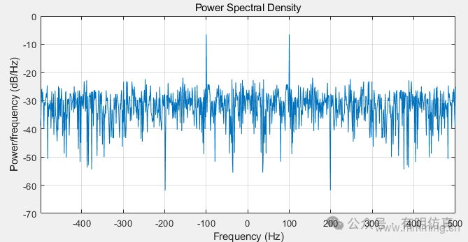
:::
If the spectrum type is specified as “psd”, the PSD estimate value is returned; if the spectrum type is specified as “power”, the power spectrum is returned.
Use the “Power” option to estimate the power of a sine wave at a specific frequency.
Create a 100 Hz sine wave with a duration of one second, sampled at 1 kHz. The amplitude of the sine wave is 1.8, corresponding to a power of 1.8 / 2 = 1.62. Use the “Power” option to estimate the power.
t = 0:1/fs:1-1/fs;
x = 1.8*cos(2*pi*100*t);
[pxx,f] = periodogram(x,hamming(length(x)),length(x),fs,'power');
[pwrest,idx] = max(pxx);
fprintf('The maximum power occurs at %3.1f Hz\n',f(idx))

fprintf('The power estimate is %2.2f\n',pwrest)

>>The maximum power occurs at 100.0 Hz
>>The power estimate is 1.62