Optimization of Cutting Parameters for Gear Discs Based on SVM and NSGA-II

1. Problem Background and Core Idea

Core Issue: In the machining of gear discs (or other parts), we need to select a set of optimal cutting parameters (usually including cutting speed (v_c), feed rate (f), cutting depth (a_p) etc.) to simultaneously optimize multiple objectives, such as:

Minimizing surface roughness (Ra) -> Improving product quality
Maximizing material removal rate (MRR) -> Increasing production efficiency
Minimizing cutting force (Fc) or tool wear -> Extending tool life and reducing costs

These objectives are often conflicting (for example, increasing the feed rate to improve MRR may lead to worse surface roughness). Therefore, this is a typical multi-objective optimization problem (MOOP).

Core Idea:

SVM (Surrogate Model): Cutting experiments (whether actual machining or finite element simulation) are costly and time-consuming. We cannot conduct thousands of experiments for the optimization algorithm to directly call. The role of SVM is to serve as a surrogate model or approximation model. We train the SVM with relatively few experimental data so that it can quickly and accurately predict the machining results (such as Ra, MRR, Fc) under given cutting parameters.
NSGA-II (Optimization Engine): NSGA-II is a powerful multi-objective genetic algorithm. Its task is to perform a global search in the parameter space to find the parameter combinations that best balance multiple conflicting objectives (i.e., the Pareto optimal solution set). It calls the SVM model to evaluate the performance of each candidate parameter set instead of conducting real experiments, greatly improving optimization efficiency.

2. Method Implementation Steps

The entire optimization process can be divided into the following key stages:

Stage One: Data Preparation and SVM Model Construction

Step 1: Experimental Design (DOE)

Objective: To obtain as representative data as possible with the least number of experiments.
Method: Use Latin Hypercube Sampling (LHS) or full factorial design methods to select N sample points within your cutting parameter space (v_c, f, a_p).
Output: A N x 3 parameter matrix.

Step 2: Data Collection

Conduct actual cutting experiments or high-fidelity simulations for each parameter combination from Step 1, measuring and recording the corresponding output responses: surface roughness (Ra), material removal rate (MRR, can be calculated as MRR = v_c * f * a_p), cutting force (Fc), etc.
Output: A N x M response matrix (M is the number of objectives).

Step 3: Data Preprocessing and SVM Training

Data Normalization: Normalize the input parameters and output responses to the range [0, 1] or [-1, 1], which is crucial for SVM performance.
Model Training:

Train an independent SVM regression model (SVR) for each output response (such as Ra, Fc).
Input: Normalized cutting parameters (v_c, f, a_p)
Output: Corresponding response values (such as Ra values)
Hyperparameter Tuning: Use grid search and cross-validation to select the optimal kernel function (commonly RBF kernel), penalty coefficient C, and kernel coefficient gamma for each SVM model.

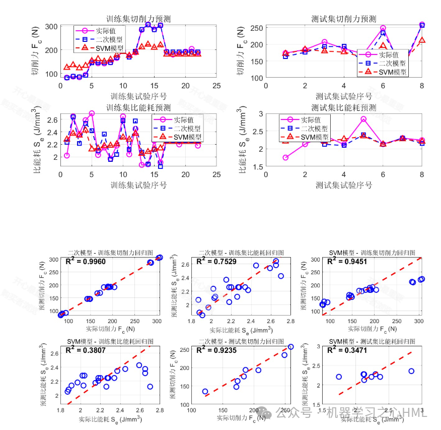
Model Validation: Validate the prediction accuracy of the SVM model using a test dataset that was not involved in training (e.g., using R², RMSE metrics). Ensure the model is reliable enough for subsequent optimization.

Stage Two: NSGA-II Multi-Objective Optimization

Step 4: Define the Optimization Problem

Decision Variables:v_c, f, a_p (need to define the upper and lower limits of the variables)
Objective Functions:

Minimize: f1 = SVM_Ra(v_c, f, a_p) (predicted surface roughness)
Maximize: f2 = MRR(v_c, f, a_p) = v_c * f * a_p (can be directly calculated)
Minimize: f3 = SVM_Fc(v_c, f, a_p) (predicted cutting force)

Constraints (optional): For example, machine power limits, maximum cutting force constraints, etc.

Step 5: Run NSGA-II Optimization

Initialization: Randomly generate an initial population (a set of cutting parameter combinations).
Iterative Optimization:

Evaluation: For each individual in the population (each set of parameters), call the SVM model trained in Step 3 to predict its f1 (Ra) and f3 (Fc), and directly calculate f2 (MRR).
Non-Dominated Sorting & Crowding Distance Calculation: The core steps of NSGA-II, sorting the population based on objective function values, distinguishing superior and inferior individuals, and maintaining diversity in the solution set.
Selection, Crossover, Mutation: Generate a new generation of the population.
Loop: Repeat Steps 1-3 until the maximum number of iterations is reached or other termination conditions are met.

Step 6: Result Analysis and Decision Making

Output: NSGA-II will ultimately output a Pareto Optimal Solution Set. This solution set is a series of optimal trade-offs, where no solution is strictly superior to another in all objectives.
Visualization: Plot the Pareto front graph (e.g., a 2D graph of Ra vs. MRR) to intuitively display the trade-offs between objectives.
Final Selection: Engineers can select the most suitable cutting parameter scheme from the Pareto solution set based on actual production needs (e.g., prioritizing quality or efficiency).

3. Key Advantages and Considerations

Advantages:

High Efficiency: Avoids a large number of physical experiments; the optimization process is completed computationally.
High Precision: The SVM model can capture complex nonlinear relationships.
Global Optimal: NSGA-II can effectively search the entire parameter space to find the global Pareto optimal solution.
Provides Multiple Choices: Offers a range of optimal solutions rather than a single solution, supporting decision-making.

Considerations:

Data Quality Determines Upper Limit: The accuracy of the SVM model heavily relies on the quality and quantity of the initial experimental data. Poor data can lead to incorrect predictions and optimization results.
SVM Hyperparameter Tuning: Needs to be done carefully; otherwise, the model may underfit or overfit.
Variable Range: The search range of NSGA-II should be within or slightly beyond the range covered by the experimental data; going too far beyond may lead to unreliable SVM predictions.

4. Code

# 1. Data Preprocessing
# 2. Define Multi-Objective Optimization Problem
# 3. Set Up and Run Optimization Algorithm
# 4. Obtain Pareto Optimal Solution Set
# 5. Select Best Solution and Validate (Subsequent Steps)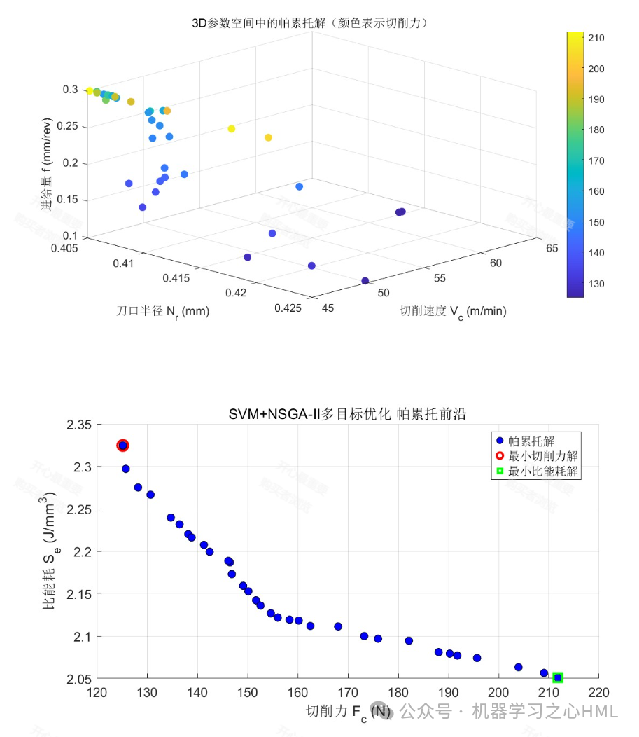

Code Acquisition

Code acquisition (non-public, please do not disturb)