In the field of machine learning, Multi-Layer Perceptron (MLP) is a fundamental Artificial Neural Network (ANN) model, which is a prototype of “deep feedforward neural networks” and is also the core foundation for understanding deep learning (such as CNNs and Transformers). It simulates the connection patterns of human neurons to fit and predict complex nonlinear data, and is widely used in tasks such as classification, regression, and feature learning.
1. Core Definition and Essence of MLP
The essence of MLP is **”multi-layer fully connected neural network”**, with two core features:
- Multi-layer structure that includes at least three layers: “input layer, hidden layer, output layer” (the hidden layer can be multiple layers, and when the number of layers is ≥2, it can be called “deep MLP”);
- Fully connected where each neuron in adjacent layers is connected to all neurons in the next layer (i.e., “fully connected layer”).
It addresses the pain point of “single-layer perceptrons being unable to handle nonlinear problems” (such as the XOR problem) — by introducing hidden layers and nonlinear activation functions, enabling the model to fit complex nonlinear mappings.
2. Breakdown of MLP Network Structure
The structure of MLP is presented in a “layered chain” format, with clear functions for each layer. Below is an analysis of the standard three-layer MLP structure:
| Layer | Core Function | Neuron Role | Key Parameters |
|---|---|---|---|
| Input Layer | Receives raw data | Only transmits input features without computation (can be viewed as a “data interface”) | Number of neurons = dimensionality of input features (e.g., when predicting house prices, features are “area, number of rooms”, so the number of input layer neurons = 2) |
| Hidden Layer | Extracts data features | Performs “weighted summation + nonlinear transformation” on the input layer signals, gradually abstracting higher-order features | Number of neurons can be customized (needs to be optimized through parameter tuning; too few leads to underfitting, too many leads to overfitting); can set multiple layers (e.g., 2 layers, 3 layers of hidden layers) |
| Output Layer | Outputs prediction results | Final processing of the high-order features from the hidden layer, outputting the required format for the task | Number of neurons = dimensionality of the task target (e.g., for binary classification tasks, the number of output layer neurons = 1; for 10-class classification tasks, it = 10) |
Structural Example: MLP Solving the XOR Problem
The XOR (exclusive or) is a classic nonlinear problem (which cannot be solved by a single-layer perceptron). MLP can solve it with “1 input layer + 1 hidden layer + 1 output layer”:
- Input layer: 2 neurons (receiving the two input features x1, x2 of XOR);
- Hidden layer: 2 neurons (transforming linear signals into nonlinear through activation functions);
- Output layer: 1 neuron (outputting the prediction result of XOR, either 0 or 1).
3. Working Principle of MLP (Forward Propagation)
The prediction process of MLP is called “Forward Propagation”, where signals flow from the input layer to the output layer, following the logic of “weighted summation → activation function transformation” at each step. The specific steps are as follows (taking a three-layer MLP as an example):
1. Input Layer: Receives Raw Features
Let the input features be a vector X = [x1, x2, …, xn] (n is the dimensionality of input features), which is directly transmitted to the hidden layer.
2. Hidden Layer: Feature Abstraction (Core Step)
Each neuron in the hidden layer processes the input signal in two steps:
-
Step 1: Weighted Summation calculates the sum of the product of input features and “connection weights”, plus the “bias term”, resulting in a “linear output”:
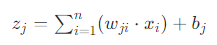
Where:
- wji is the connection weight from the i-th neuron of the input layer to the j-th neuron of the hidden layer (a core learnable parameter);
- bj is the bias term of the j-th neuron in the hidden layer (compensating for “signal offset when input is 0”, also a learnable parameter);
- zj is the linear output of the j-th neuron in the hidden layer.
-
Step 2: Nonlinear Activation uses an “activation function” to transform zj, introducing nonlinearity (otherwise, multiple layers would be equivalent to a single layer), resulting in the final output of the hidden layer aj: aj = f(z_j) Common activation functions
3. Output Layer: Generates Prediction Results
The output of the hidden layer (A = [a_1, a_2, …, a_m]) (m is the number of neurons in the hidden layer) serves as the input to the output layer, repeating the “weighted summation → activation function” steps, but the activation function needs to be adjusted according to the task:
- Binary Classification Task has 1 neuron in the output layer, using Sigmoid activation (outputting probability values, e.g., > 0.5 predicts 1, otherwise 0);
- Multi-class Classification Task has k neurons in the output layer (k is the number of classes), using Softmax activation (outputting the probability of each class, with probabilities summing to 1);
- Regression Task has 1 neuron in the output layer, not using an activation function (directly outputting continuous values, such as predicting house prices or temperatures).
4. Core of MLP Training: Backpropagation
The “learning process” of MLP is essentially optimizing the “connection weights w” and “biases b” through backpropagation, aiming to minimize the “error between predicted values and true values” (such as Mean Squared Error (MSE), Cross-Entropy Loss (CE)).
The core logic of backpropagation:
- Calculate Loss using a loss function (such as MSE, CE) to compute the error between the predicted values of the output layer and the true labels;
- Backpropagate Gradients
- Using the “chain rule” to backpropagate the error from the output layer to the input layer, calculating the gradient of each parameter (w, b) with respect to the loss (i.e., “how parameter changes affect loss”);
- Update Parameters using an optimizer (such as gradient descent, Adam) to adjust parameters based on the gradients, reducing the loss.
This process iterates repeatedly until the loss converges to a minimum value, completing the training of the model.
5. Advantages and Disadvantages of MLP
Advantages:
- Strong Nonlinear Fitting Ability through hidden layers and activation functions, can fit any complex nonlinear data (theoretically, 1 hidden layer is sufficient to fit any continuous function, known as the “Universal Approximation Theorem”);
- Simple and Understandable Structure compared to CNNs and Transformers, the layered fully connected structure of MLP is easier to understand, making it the best case for beginners in neural networks;
- Basic Generalization can alleviate overfitting through regularization (such as Dropout, L2 regularization), adapting to different tasks (classification, regression, recommendation, etc.).
Disadvantages:
- Large Number of Parameters due to the fully connected nature, leading to excessive parameters (e.g., if the input layer has 1000 dimensions and the hidden layer has 1000 neurons, just the weights of this layer exceed 1 million), making it prone to overfitting and low training efficiency;
- Lack of Feature Locality the fully connected structure does not consider the spatial/temporal relationships of input features (such as pixel neighborhoods in images, word order in text), thus performing much worse than CNNs and RNNs in image and NLP tasks;
- Risk of Gradient Vanishing when there are too many hidden layers, the gradients during backpropagation can diminish with the number of layers (especially when using Sigmoid activation), making it difficult to update parameters in deep layers.
6. Typical Application Scenarios of MLP
Although MLP has been replaced by more specialized models in complex structured data (such as images and text), it still has wide applications in the following scenarios:
- Traditional Machine Learning Tasks such as classification of structured data (customer churn prediction), regression (sales forecasting), especially when the feature dimensionality is not high;
- Basic Module of Deep Learning as a subcomponent of complex models (e.g., the fully connected output layer of CNNs, the Feed-Forward Network of Transformers is essentially MLP);
- Simple Generation Tasks such as the generator/discriminator of Generative Adversarial Networks (GANs), and the encoder/decoder of Autoencoders (AEs), commonly using MLP structures;
- Small Scale Dataset Tasks compared to CNNs and Transformers, MLP requires less data, making it suitable for modeling small-scale datasets.
Conclusion
MLP is the “cornerstone model” of neural networks — its “multi-layer structure” and “backpropagation” concept laid the foundation for deep learning. Understanding the working principles of MLP (forward propagation, backpropagation, activation functions) is a key prerequisite for mastering more complex deep learning models (such as CNNs and Transformers). Although it has been surpassed by specialized models in specific tasks, the core logic of MLP still runs through almost all deep learning architectures.