Welcome to click “The Beauty of Algorithms and Programming” ↑ to follow us!
This article was first published on WeChat public account: “The Beauty of Algorithms and Programming”, welcome to follow us for timely updates on more articles in this series.
Welcome to join the team circle! Face-to-face with the author! Click directly!
1. Common Ideas for Plotting Graphs
Generally, the basic idea of manually plotting function graphs is to determine the range of values for the independent variable, select appropriate points for the independent variable, derive the corresponding values for the dependent variable through the function expression, and connect these points to obtain a rough graph.
Using Matlab to plot function graphs follows the same idea; the more points you take for the independent variable, the closer the shape connecting these points will be to the actual function graph.
2. Common Language Specifications and Plotting Functions in Matlab
In Matlab, selecting independent variable operations becomes extremely simple, with the general format as follows: X = lower limit: interval: upper limit. For detailed information, please refer to the case study. Matlab’s representation of functions is also very close to natural language, and case studies can be referred to for learning. When plotting graphs, Matlab has different functions for two-dimensional and three-dimensional graphs. The function generally used for plotting two-dimensional graphs is the “plot” function; when calling it, you only need to provide the corresponding independent and dependent variables, for example, plot(x,y) plots the function graph where x is the independent variable and y is the dependent variable; for three-dimensional graphs, the “surf” function is generally used, which is used similarly to the “plot” function. Of course, these two plotting functions also have some more advanced usages, which will not be introduced one by one here.
3. Precautions
Since there are two methods for matrix multiplication in Matlab, one is matrix multiplication, which follows the rules of matrix multiplication, represented by the “*” symbol; the other is element-wise multiplication of matrices, which requires the dimensions of the matrices to be the same, resulting in a matrix of the same dimension where each value is the result of the corresponding elements multiplied, represented by the “.*” symbol. At the same time, when plotting two-dimensional graphs, the plot function does not use grid lines by default, so you need to add grid lines using the “grid” function. In function expressions that contain division, you should also avoid exceptional cases where the divisor is zero; a common solution is to add an eps (infinitesimal) after the divisor part of the expression.
4. Case Study for Graph Plotting
Plotting a two-dimensional function graph: The function graph in (0,4):
|
x=0:pi/50:4*pi; y=exp(-t/3).*sin(3*t); plot(x,y); grid |
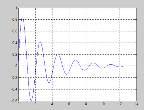
Figure 4.1 Two-Dimensional Function Graph
Plotting a three-dimensional function graph:
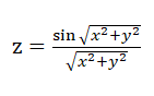
For the function graph, x,y the range of values is [-8,8]:
|
x=-8:0.5:8;#Determine x‘s range of values y=x’; X=ones(size(y))*x;#Since this is a three-dimensional graph, at this time, X is no longer a one-dimensional array, but a two-dimensional array, part of the results are as follows Y=y*ones(size(x));#Similar to X R=sqrt(X.^2+Y.^2)+eps;#Exception handling Z=sin(R)./R; surf(X,Y,Z) |
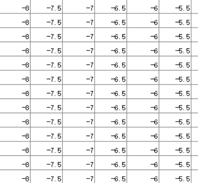
Figure 4.2 Three-Dimensional Function Independent Variable X Representation
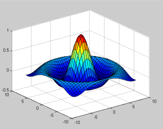
Figure 4.3 Three-Dimensional Function Graph
END
Editor | Wang Wenxing
Responsible Editor | Huang Zhangyu
The greater the ability, the greater the responsibility. Be pragmatic and meticulous.
——where2go Team
WeChat ID: The Beauty of Algorithms and Programming

Long press to identify the QR code to follow us!
Warm Reminder: Click the lower right corner of the page “Write a Message” to leave a comment, looking forward to your participation! Looking forward to your forwarding!