
1. Understanding MATLAB
1. Overview of MATLAB
(1) In universities in Europe and America, MATLAB has become a fundamental teaching tool for courses such as linear algebra, automatic control theory, digital signal processing, time series analysis, dynamic system simulation, and image processing. It has become a basic skill that undergraduate, master’s, and doctoral students must master.
(2) In design research institutions and industrial sectors, MATLAB has been widely used to research and solve various specific engineering problems.
(3) It can be anticipated that MATLAB will play an increasingly important role in scientific research and engineering applications in our country.
2. Features of MATLAB
Powerful functionality
-
Advantages of numerical computation
-
Advantages of symbolic computation
-
Powerful 2D and 3D data visualization capabilities
Many functional functions with algorithm adaptability
-
MATLAB uses arrays as the basic unit of computation
-
Has a large number of algorithm optimization functional functions
-
Easy programming, high efficiency
Simple language, rich content
-
The language and writing form are very close to conventional mathematical writing
-
Complete help system, easy to learn and use
MATLAB Main Page
3. Using the Command Window
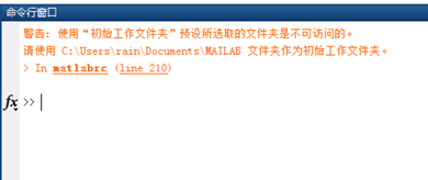
MATLAB Command Window
“>>” along with the blinking cursor indicates that the system is ready and waiting for input;
Press the 【Enter】 key in the command line window to submit the command for execution;
Calculate 2+[(13-7)×8]÷23
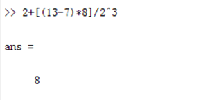
The operators used in MATLAB (such as addition, subtraction, multiplication, and division) are common in various computational programs;
The “ans” in the calculation result is the abbreviation of the English word “answer” and is a predefined variable in MATLAB;
4. Creating M Files
When a few lines of code cannot complete a task, it is necessary to create an M script, placing all code in one script file to execute in order.
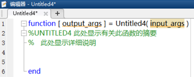
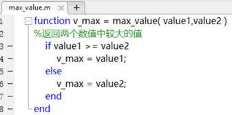
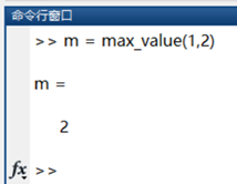
Click to create a new file, selecting either a new script or a new function. Script files can be executed directly, while function files need to be called from a script file or the command line window before they can be used.
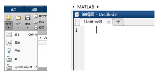
The newly created function file comes with default return variables, parameters, and function names, which can be modified as needed, and the code can be edited within the function body.
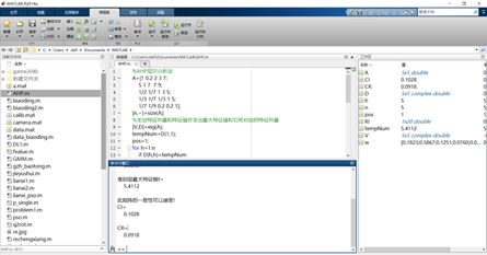
5. Directory and File Management
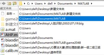
The current folder contains a detailed file list under the working directory, allowing for the selection of running M files, loading mat data, and editing files. To run, simply right-click to open.
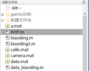
To change the current working directory, click the drop-down arrow on the right and reselect.
In MATLAB, all files are managed through a rigorous directory folder structure. When searching for files, functions, and data, MATLAB will search according to a predetermined search path. The order of checks is generally as follows: first, check if the content being searched for is a variable; if it is not a variable, then check if it is a built-in function; if it is neither a built-in function nor a variable, then check if there are M files in the current working directory. If not, it will search in other specified paths.
6. Managing Search Paths
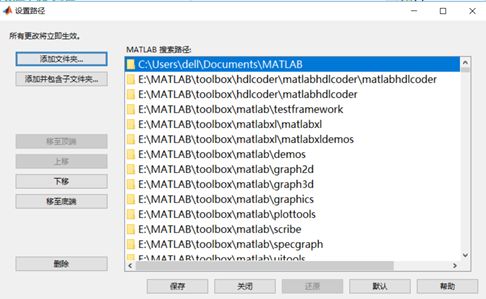
If users have multiple files that need to interact with MATLAB or frequently need to exchange data, they can place these files on MATLAB’s search path to ensure they can be called from the search path. If a directory needs to run generated data and files, it must be set as the current working directory. If users need to modify the search path, they can enter the command pathtool in the command line window.
Users can click “Add Folder” to add a new path to the search path. If the path to be searched also contains subfolders, click “Add and Include Subfolders”.
If users need to adjust the search order of already added folders in the search path, they can use the buttons “Move to Top”, “Move Up”, “Move Down”, and “Move to Bottom” to change the folder’s position.
2. Basic Knowledge of MATLAB
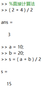
1. Simple Calculations in MATLAB
When variable names are not defined, data temporarily resides in ans. After defining variables, their meanings are clear, and the calculation process is straightforward.
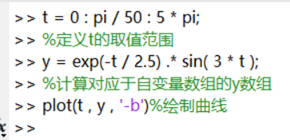
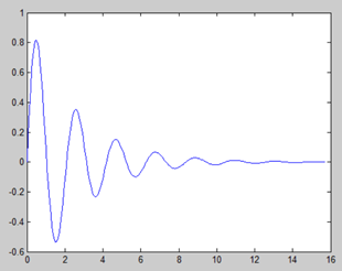
Using MATLAB, it is easy to compute and plot function curves.
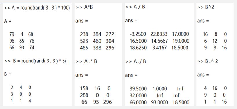
2. Basic Operators
The order of precedence for mathematical processing in MATLAB is consistent with the usual order of mathematical processing. Exponents take precedence; multiplication and division follow; parentheses can change precedence, and expressions are evaluated from left to right.
3. Numbers, Variables, and Expressions
Number description:
MATLAB numbers use the conventional decimal representation, can have decimal points and negative signs, and default to double-precision floating-point data.
For example: 3 -10 0.001 1.3e10 1.1343e-6
Variable naming rules:
1. Variable names and function names are case-sensitive;
2. Variable names can contain letters, underscores, and numbers but must start with a letter;
3. Variable names can contain a maximum of 63 characters.
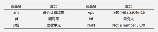
Predefined variables in MATLAB:
4. Arrays
(1) Generating Arrays
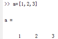
One-dimensional arrays
1. Direct input method: separate array elements with spaces, commas, and semicolons to generate a one-dimensional array.
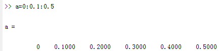
2. Step generation method: x = a : step : b
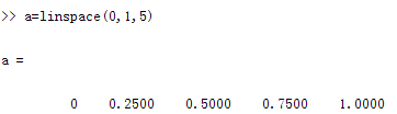
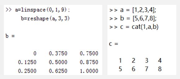
3. Equidistant linear generation method: x = linspace(a, b, n), generates n sampling points in the interval from a to b.
Two-dimensional arrays
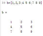
1. Direct input method: separate elements in the same row with commas or spaces, and separate different rows with semicolons.
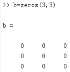
2. Call built-in functions, such as zeros, ones, rand, etc.
3. Low-dimensional array conversion, converting low-dimensional arrays into high-dimensional arrays using functions like reshape, cat, etc.
(2) Accessing Arrays
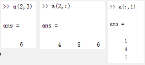
a=[1 2 3;4 5 6;7 8 9];
a(2,3) a(2,:) a(:,1)
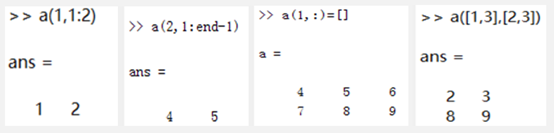
a(1,1:2) a(2,1:end-1) a(1,:)=[] a([1,3],[2,3])
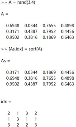
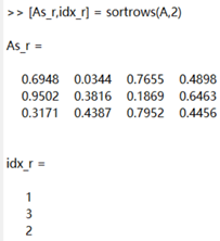
Sorting function:
[As,idx] = sort(A)
[As_r,idx_r] = sortrows(A)
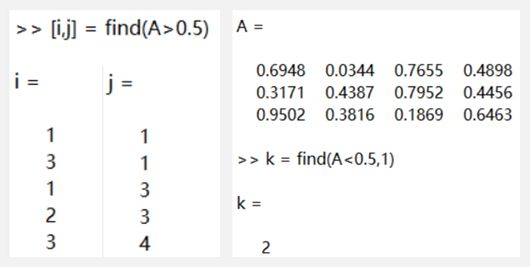
Sub-array search
[i,j] = find(A>0.5)
k = find(A>0.5,1)
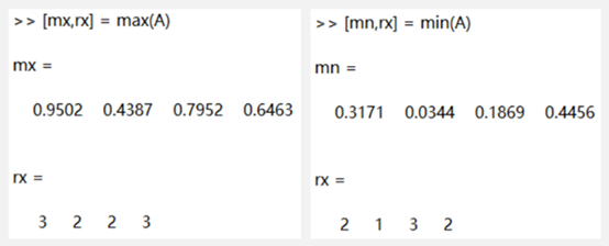
Maximum and minimum value search
[mx,rx] = max(A)
[mn,rx] = min(A)
3. Programming Basics
1. Control Flow
(1) For Loop Structure
In a for loop structure, a certain loop condition must be set, and MATLAB executes the commands within the loop body according to the set number of loops.
for x = array
commands
end
Here, x is the loop variable, array is the condition array, and commands are the loop code to be executed. The number of times the loop body executes is determined by the array.
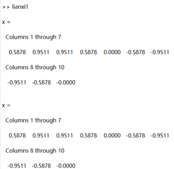
% Example of for loop structure
for n = 10 : -1 : 1
x(n) = sin(n * pi / 5);
end
x
array = ceil(rand(1,10) * 10);
for n = array
x(n) = sin(n * pi / 5);
end
x
(2) While Loop Structure
The while loop structure performs an infinite number of loop operations until the loop body meets the end condition or reaches a certain number of loops.
while expression
commands
end
Here, expression is the condition expression, which is generally a scalar result but can also be an array expression. When the scalar result is true, the loop body continues to execute; when the result of the expression is an array, the loop body is executed only when all elements in the array are true.
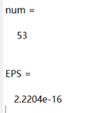
% Example of while loop structure
% Calculate the precision of floating-point number eps
EPS = 1;
num = 0;
while (EPS + 1 ) > 1
EPS = EPS / 2;
num = num + 1;
end
num
EPS = EPS * 2
(3) If Statement Structure
The if statement structure determines different commands based on a given condition.
if-else-end statement structure
Executes different command lines based on whether the judgment condition is true or false.
if expression
commands
end
if expression
commands1
else
commands2
end
When expression contains multiple sub-logic expressions, MATLAB uses “short-circuit” evaluation for each expression, for example (expression1 | expression2), where expression2 is only evaluated if expression1 is false.
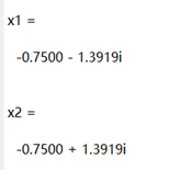
% Example of if statement structure
% Find the roots of the quadratic equation a*x^2 + b*x + c = 0
a = 2; b = 3; c = 5;
delta = b^2 – 4*a*c;
if delta > 0
x1 = (-b+sqrt(delta))/(2*a)
x2 = (-b-sqrt(delta))/(2*a)
elseif delta == 0
x1 = (-b+sqrt(delta))/(2*a)
else
real_a = -b/(2*a);
imag_b = sqrt(abs(delta)) / (2*a);
x1 = real_a – imag_b*i
x2 = real_a + imag_b*i
end
2. Control Commands
When writing MATLAB M files, various control flow structures are often used. During the execution of these flow structures, it is often necessary to terminate loops or jump out of subprograms in advance, which requires the use of control statements. Here, we mainly introduce commonly used continue and break statements.
The continue command is mainly used in loop statements to prematurely end the current operation of the loop body, placing continue directly within the loop control body to work with if statement.
The break command, like the continue command, is used in loop structures. When the break command is executed, the program exits the loop structure and moves to the next statement outside the loop.
The continue command jumps to the end of the loop statement to end one iteration of the loop, while the break command exits the loop body where break is located.
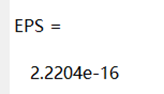
% Example of continue and break control statements
% Calculate the precision of the floating-point number eps
EPS = 1;
for n = 1:1000
EPS = EPS / 2;
if (1 + EPS ) >1
continue
end
EPS = EPS * 2;
break;
end
EPS
3. Concept of Program Vectorization
Vectorization processing is a special concept in MATLAB, which refers to using vectorized statements to replace loop structures. Due to vectorization processing, data is pre-allocated memory, resulting in significantly faster execution speed.
Example of program vectorization
Calculating the square of each element of an array using both vectorization and loop structures.
% Loop structure
for i = 1:100
s1(i) = i^2;
end
% Vectorized processing
s2 = [1:100].^2;
% Loop structure
tic
num_max = 1000000;
for i = 1:num_max
s1(i) = i^2;
end
toc
% Vectorized processing
tic
s2 = [1:num_max].^2;
toc
4. Logical Arrays and Vectorization
In addition to basic numerical data types and strings, logical data is also a type of data. Logical data can be created through relational and logical expressions or by using the logical command to create logical arrays.
Logical arrays play a very important role in the process of vectorization, allowing us to use logical arrays to complete the vectorization process.
% Loop structure
tic
num_max = 1000000;
for i = 1:num_max
if i < 500000
s1(i) = i^2;
else
s1(i) = i;
end
end
toc
% Vectorized processing
tic
a = 1:num_max;
s2 = a(a<500000).^2;
toc
Past Recommendations
MATLAB Advanced Tutorial | Extracting Brightness from Black and White Photos to Create Color Maps
MATLAB Introduction Tutorial | Long-term Investment Compound Interest Problem
MATLAB Introduction Tutorial | 001 Volume of a Sphere Problem
Installation Tutorial | MATLAB 2016b~2018b Installation Guide