1. Two-Dimensional Data Curve Plotting
1.1 Basic Function for Drawing 2D Curves
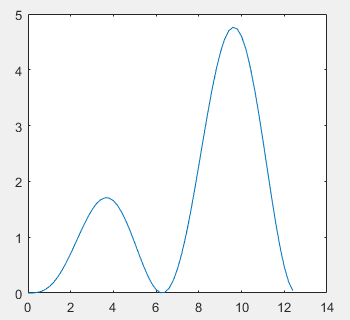
The plot() function is used to draw linear coordinate curves on a two-dimensional plane. It requires a set of x coordinates and corresponding y coordinates to plot a 2D curve with x and y as the horizontal and vertical axes, respectively. Example:
t=0:0.1:2*pi;
x=2 * t;
y=t.*sin(t).*sin(t);
plot(x, y);
Copy
2. Plot Function with Multiple Input Parameters
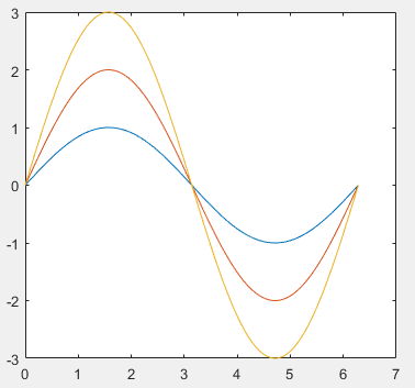
The plot function can include several pairs of vectors, each group can plot a curve. The calling format for the plot function with multiple input parameters is: plot(x1, y1, x2, y2, …, xn, yn) Example:
x=linspace(0,2*pi,100);
plot(x,sin(x),x,2*sin(x),x,3*sin(x))
Copy
3. Plot Function with Options
MATLAB provides several plotting options to determine the line style, color, and data point marker symbols of the curves. These options are shown in the table below:
|
Line Style |
Color |
Marker Symbol |
|
|---|---|---|---|
|
– Solid Line |
b Blue |
. Point |
s Square |
|
: Dashed Line |
g Green |
o Circle |
d Diamond |
|
.- Dash-Dot Line |
r Red |
x Cross |
v Downward Triangle |
|
— Double Dash Line |
c Cyan |
+ Plus |
^ Upward Triangle |
|
m Magenta |
* Star |
< Left Triangle |
|
|
y Yellow |
Right Triangle |
p Pentagon |
|
|
k Black |
h Hexagon |
||
|
w White |
Example: Use different line styles and colors to draw curves and their envelopes on the same coordinate.
x=(0:pi/100:2*pi)';
y1=2*exp(-0.5*x)*[1,-1];
y2=2*exp(-0.5*x).*sin(2*pi*x);
x1=(0:12)/2;
y3=2*exp(-0.5*x1).*sin(2*pi*x1);
plot(x,y1,'k:',x,y2,'b--',x1,y3,'rp');
Copy
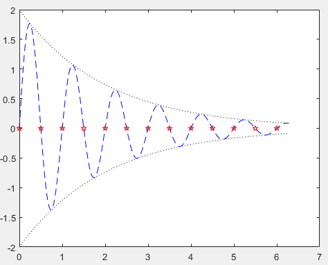
In this plot function, three sets of plotting parameters are included: the first set uses a black dashed line to draw two envelope lines, the second set uses a blue double dashed line to draw curve y, and the third set uses red pentagons to mark discrete data points.
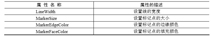
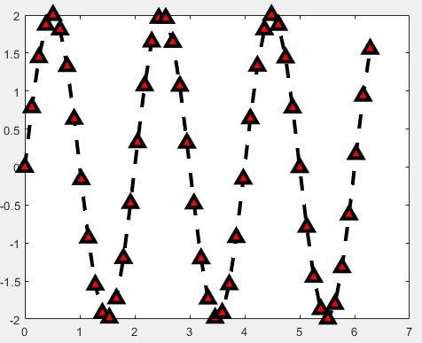
Example: Set the line width of the sine curve to 3, use upward triangles to mark data points, set the edge color of the markers to black, set the fill color of the markers to red, and set the marker size to 10. The MATLAB code is as follows:
% X-Axis
x = linspace(0, 2*pi, 50);
% Generate data points, Y-Axis
y = 2 * sin(pi * x);
% Plotting
figure
% Set line width to 3
plot(x, y, 'k--^', 'LineWidth', 3, ...
  'MarkerEdgeColor', 'k', ... % Set marker edge color to black
  'MarkerFaceColor', 'r', ... % Set marker fill color to red
  'MarkerSize', 10)  % Set marker size to 10
Copy
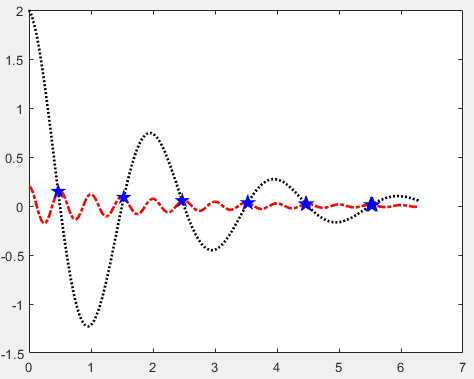
Example: Use pentagons to mark the intersection points of the two curves.
% X-Axis
x = linspace(0, 2*pi, 1000);
% Generate data points, Y-Axis
y1 = 0.2 * exp(-0.5 * x).* cos(4 * pi * x);
y2 = 2 * exp(-0.5 * x) .* cos(pi * x);
% Find indices where y1 and y2 are approximately equal
k = find( abs(y1-y2) < 1e-2 );
% Take x coordinates where y1 and y2 are equal
x1 = x(k);
% Calculate y coordinates where y1 and y2 are equal
y3 = 0.2 * exp(-0.5 * x1) .* cos(4 * pi * x1);
% Plotting
figure
plot(x, y1, 'r-.', x, y2, 'k:', x1, y3, 'bp','LineWidth',2);
Copy
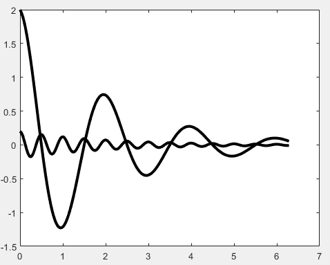
4. Dual Y-Axis Function plotyy
In MATLAB, if you need to plot two graphs with different vertical scales, you can use the plotyy function. This function can plot two functions with different dimensions and orders of magnitude on the same coordinate, which is helpful for comparative analysis of graphical data. The format is: plotyy(x1,y1,x2,y2) where x1,y1 corresponds to one curve and x2,y2 corresponds to another curve. The x-axis scale is the same, but there are two y-axes, with the left corresponding to the data pair x1,y1 and the right corresponding to x2,y2.
x=0:pi/100:2*pi;
% Generate curves
y1=0.2*exp(-0.5*x).*cos(4*pi*x);
y2=2*exp(-0.5*x).*cos(pi*x);
% Plotting
figure
plotyy(x,y1,x,y2);
plot(x, y1, 'k-', x, y2, 'k-', 'LineWidth', 3)
Copy
1.2 Auxiliary Operations for Plotting
1. Graph Annotation
title('Graph Title')
xlabel('X-Axis Label')
ylabel('Y-Axis Label')
text(x,y,'Graph Description')
legend('Legend 1','Legend 2',…)
Copy
The title, xlabel, and ylabel functions are used to describe the names of the graph and axes.
The text function adds a description at the coordinate point (x,y).
The legend function is used to draw legends for the line styles, colors, or data point markers used in the curves. The legend is placed in a blank area, and users can also move the legend with the mouse to the desired position.
Except for the legend function, the other functions also apply to three-dimensional graphs, where the z-axis description is used with the zlabel function.
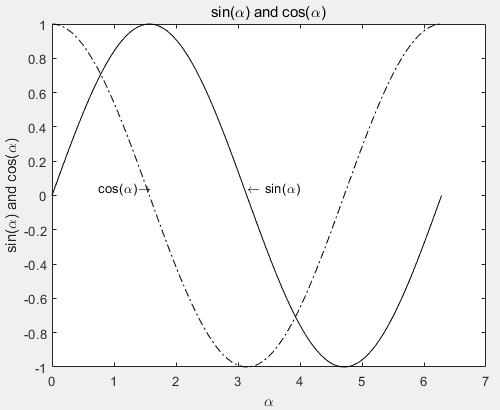
Example: Draw sine and cosine curves, set the graph title, and label the x and y axes, and set the curve legend.
% X-Axis
x=0:pi/50:2*pi;
% Curve data
y1=sin(x);
y2=cos(x);
% Plotting
figure
plot(x, y1, 'k-', x, y2, 'k-.')
% Text annotation
text(pi, 0.05, '\leftarrow sin(\alpha)')
text(pi/4-0.05, 0.05, 'cos(\alpha)\rightarrow')
% Title annotation
title('sin(\alpha) and cos(\alpha)')
% Axes annotation
xlabel('\alpha')
ylabel('sin(\alpha) and cos(\alpha)')
Copy
2. Coordinate Control
axis([xmin xmax ymin ymax zmin zmax]) If only the first four parameters are given, the coordinate system range is selected based on the minimum and maximum values of the x and y axes to draw appropriate 2D curves. If all parameters are given, a three-dimensional graph is drawn. The axis function has rich functionality, with common usages including:
-
axis equal: Equal length scales for x and y axes -
axis square: Produce a square coordinate system (default is rectangular) -
axis auto: Use default settings -
axis off: Turn off the coordinate axis -
axis on: Show the coordinate axis -
axis tight: Display the coordinate axis range compactly, meaning the axis range is the range of plotting data -
grid on/off: Command to control whether to draw grid lines or not
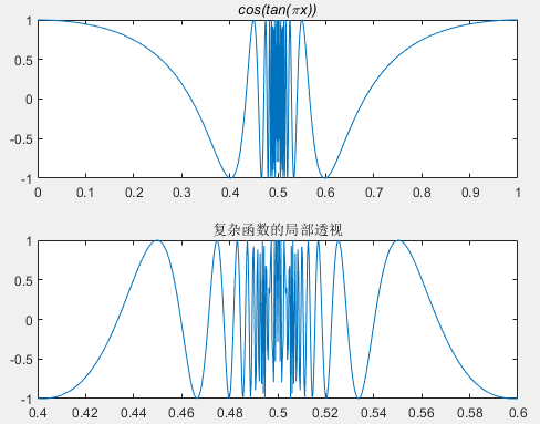
Example: Observe the curve of y=cos(tan(\pi x)) near x=0.5.
% X-Axis
x = 0:1/3000:1;
% Generate error curve
y = cos(tan(pi*x));
% Plotting
figure
% Split window into 2*1 sub-windows
subplot(2,1,1)
plot(x,y)
title('\itcos(tan(\pix))')
% Coordinate axis adjustment
subplot(2,1,2)
plot(x,y)
axis([0.4 0.6 -1 1]);
title('Local Perspective of Complex Function')
Copy
subplot(m,n,p) This function divides the current window into m×n plotting areas, m rows, each with n plotting areas, numbered in row-major order. The p-th area is the current active area. Each plotting area allows for drawing graphs with different coordinate systems separately.
1.3 Other Functions for Drawing 2D Graphs
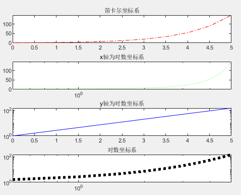
1. Logarithmic Coordinate Graph In practical applications, logarithmic coordinates are often used. MATLAB provides functions for drawing logarithmic and semi-logarithmic coordinate curves, with the following calling format:
semilogx(x1,y1,option1,x2,y2,option2,…)
semilogy(x1,y1,option1,x2,y2,option2,…)
loglog(x1,y1,option1,x2,y2,option2,…)
Copy
In these functions, the definitions of options are exactly the same as in the plot function, with the only difference being the selection of axes. The semilogx function uses semi-logarithmic coordinates, with the x-axis having a common logarithmic scale while the y-axis remains linear. The semilogy function is exactly the opposite of semilogx. The loglog function uses full logarithmic coordinates, with both x and y axes adopting logarithmic scales. Example: Draw the function y=e^x.
% X-Axis
x=0:0.5:5;
% Y-Axis
y = exp(x);
% Plotting
figure
% Cartesian coordinate system
subplot(4, 1, 1)
plot(x, y, 'r-.')
title('Cartesian Coordinate System')
% Semi-logarithmic coordinate system
subplot(4, 1, 2)
semilogx(x, y, 'g:')
title('X-Axis as Logarithmic Coordinate System')
subplot(4, 1, 3)
semilogy(x, y, 'b-')
title('Y-Axis as Logarithmic Coordinate System')
% Logarithmic coordinate system
subplot(4, 1, 4)
loglog(x, y, 'k:','LineWidth',4)
title('Logarithmic Coordinate System')
Copy
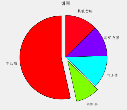
1. Pie Chart
-
pie(x): Draws a pie chart of data x, where x can be a vector or matrix, with each element representing a sector of the pie chart, and showing the proportion of each element’s total. -
pie(x, explode): Draws a pie chart of data x, where the parameter explode can be used to set a certain important sector of the pie chart to be highlighted. Note that the length of the explode vector must equal the number of elements in x and correspond to the meaning of the elements in x. Non-zero values in explode will separate the corresponding sector from the pie chart, typically set as 1. -
pie(x, labels): Draws a pie chart of data x, where the parameter labels can be used to set the display labels for each sector of the pie chart. Note that the labels parameter should be a string or a number.
Example: A graduate student has an average monthly expense of 190 yuan for living expenses, 33 yuan for materials, 45 yuan for phone bills, 42 yuan for clothing, and 45 yuan for other expenses. Please represent his monthly expense ratio in a pie chart and separate the slices for the highest and lowest expenses.
% Data Preparation
x=[190 33 45 42 45];
% Separation display settings
explode=[1 1 0 0 0];
% Plotting
figure()
colormap hsv
pie(x,explode,{'Living Expenses','Material Expenses','Phone Bills','Clothing Expenses','Other Expenses'})
title('Pie Chart')
Copy
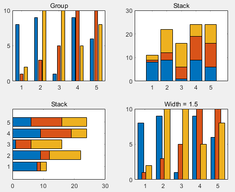
2. Bar Chart See the example:
% Random function generates a 5*3 array, rounding the generated data
Y = round(rand(5,3)*10);
% Plotting
subplot(2,2,1)
bar(Y,'group')
title 'Group'
% Stacked 2D vertical bar chart
subplot(2,2,2)
bar(Y,'stack')
title('Stack')
% Stacked 2D horizontal bar chart
subplot(2,2,3)
barh(Y,'stack')
title('Stack')
% Set the width of the bars to 1.5
subplot(2,2,4)
bar(Y,1.5)
title('Width = 1.5')
Copy
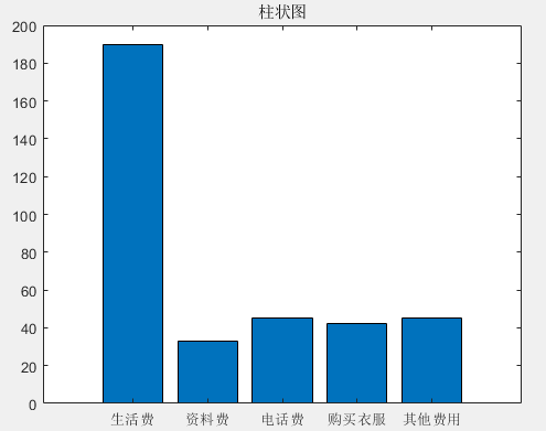
Example: A graduate student has an average monthly expense of 190 yuan for living expenses, 33 yuan for materials, 45 yuan for phone bills, 42 yuan for clothing, and 45 yuan for other expenses. Please represent his monthly expense ratio in a bar chart. The MATLAB code is as follows:
% Data Preparation
y=[190 33 45 42 45];
x=1:5 ;
% Plotting
figure
bar(x,y)
title('Bar Chart');
set(gca,'xTicklabel',{'Living Expenses','Material Expenses','Phone Bills','Clothing Expenses','Other Expenses'})
Copy
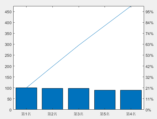
3. Pareto Chart A Pareto chart consists of a horizontal axis, two vertical axes, multiple bars arranged in descending order, and a line representing cumulative frequency. This chart can effectively analyze the importance of various factors and can be used to identify major problems or causes. In MATLAB, the pareto() function is used to draw a Pareto chart, with the following calling format: pareto(y): Draws a Pareto chart of data y. The height of the bars in the Pareto chart represents the size of the y values. pareto(y,x): Draws a Pareto chart of data y. When x is numeric, it specifies the numerical horizontal axis. When x is a string, it specifies the string type horizontal axis.
Y=[100 98 97 90 90];
names={'1st Place' '2nd Place' '3rd Place' '4th Place' '5th Place'};
pareto(Y,names)
Copy
2. Three-Dimensional Graphs
2.1 Drawing 3D Curves
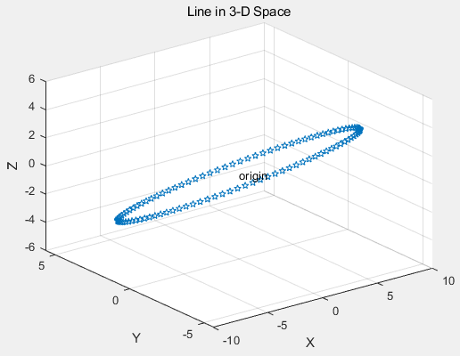
1. Use the plot3() function to draw 3D curves. The most basic 3D graph function is plot3, which extends the functionalities of the 2D plotting function plot to three-dimensional space and can be used to draw 3D curves. Its calling format is: plot3(x1,y1,z1,option1,x2,y2,z2,option2,…) where each group of x, y, z forms a set of curve coordinate parameters, and the definition of options is the same as that of plot. When x, y, z are the same dimension vectors, they correspond to elements to form a 3D curve. When x, y, z are the same dimension matrices, the corresponding column elements are used to plot the 3D curve, with the number of curves equal to the number of columns of the matrix.
Example:
t=0:pi/50:2*pi;
x=8*cos(t);
y=4*sqrt(2)*sin(t);
z=-4*sqrt(2)*sin(t);
plot3(x,y,z,'p');
title('Line in 3-D Space');
text(0,0,0,'origin');
xlabel('X');ylabel('Y');zlabel('Z');grid;
Copy
2. Drawing 3D Mesh Plots In MATLAB, when drawing 3D graphs, it is often necessary to first create a 3D mesh, which means first creating a coordinate system for the planar graph. In MATLAB, the commonly used meshgrid() function generates mesh data, with the following calling format: [X,Y]=meshgrid(x,y): Used to generate mesh data from vectors x and y, transforming them into matrix data X and Y, where the rows of matrix X are vector x and the columns of matrix Y are vector y. [X,Y]=meshgrid(x): Generates mesh data from vector x, equivalent to [X,Y]=meshgrid(x,x). [X,Y,Z]=meshgrid(x,y,z): Generates 3D mesh data from vectors x, y, z, where the generated data X and Y can represent the x and y coordinates in 3D plotting.
3D mesh plots are created by connecting adjacent data points in three-dimensional space, forming a mesh. The main functions for plotting 3D mesh plots in MATLAB are mesh(), meshc(), and meshz(). Among them, the mesh() function is the most commonly used, with the following calling format: mesh(x,y,z): Draws a 3D mesh plot, where x, y, z represent the coordinates of the 3D mesh plot along the x-axis, y-axis, and z-axis, respectively, and the color of the plot is determined by matrix z. mesh(Z): Draws a 3D mesh plot, using the column and row indices of matrix Z as the x-axis and y-axis coordinates of the 3D mesh plot, respectively, with the color of the plot determined by matrix Z. mesh(...,C): Input parameter C controls the color of the drawn 3D mesh plot. mesh(...,'PropertyName',PropertyValue,...): Sets the specified property value for the 3D mesh plot.
The meshc() function can draw a 3D mesh plot with contour lines, with a calling format similar to the mesh() function, but the meshc() function does not support setting properties for the mesh lines or contour lines. The meshz() function can draw a 3D mesh plot with a bottom edge, with a calling format similar to the mesh() function, but the meshz() function does not support setting properties for the mesh lines.
Additionally, the function ezmesh(), ezmeshc(), and ezmeshz() can directly plot the corresponding 3D mesh plots based on function expressions.
Since the mesh lines are opaque, sometimes the drawn 3D mesh plot only shows the front part of the plot, while the back part may be hidden by the mesh lines and not displayed. MATLAB provides the command hidden to observe the hidden parts of the plot, with the following calling format: hidden on: Sets the hidden parts of the mesh to be invisible, which is the default state. hidden off: Sets the hidden parts of the mesh to be visible. hidden: This command toggles the visibility of the hidden parts of the mesh.
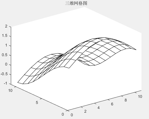
Example: Draw a simple 3D mesh plot
% Data Preparation
t=0:pi/10:pi;
x=sin(t);
y=cos(t);
[X,Y]=meshgrid(x,y);
z =X + Y;
% Plotting
figure
mesh (z,'FaceColor','W','EdgeColor','K')
grid
title('3D Mesh Plot');
Copy
2.2 Drawing 3D Surface Plots
3D surface plots can also be used to represent the variation of data in three-dimensional space. Unlike the previously discussed 3D mesh plots, surface plots fill the mesh areas with different colors. In MATLAB, the function for drawing 3D surface plots is surf(), with the following calling format: surf(Z): Draws a 3D surface plot of data Z, where the column and row indices of matrix Z are used as the x and y coordinates of the 3D mesh plot, respectively, and the color of the plot is determined by matrix Z. surf(X, Y, Z): Draws a 3D surface plot, where X, Y, Z represent the coordinates of the 3D mesh plot along the x-axis, y-axis, and z-axis, respectively, with the color determined by matrix Z. surf(X, Y, Z, C): Draws a 3D surface plot, where input parameter C controls the color of the drawn 3D surface plot. surf(..., 'PropertyName', PropertyValue): Draws a 3D surface plot, setting the corresponding property values.
The function surfc() is used to draw a 3D surface plot with contour lines, with a calling format similar to the surf() function. The function surfl() can be used to draw a 3D surface plot with lighting effects, with a different calling format than surf() and surfc().
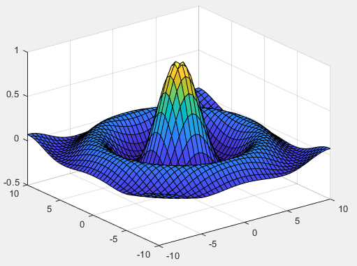
Example: A simple example of the surf() function
% Data Preparation
xi=-10:0.5:10;
yi=-10:0.5:10;
[x,y]=meshgrid(xi,yi);
z=sin(sqrt(x.^2+y.^2))./sqrt(x.^2+y.^2);
% Plotting
surf(x,y,z)
Copy
2.3 Drawing 3D Slice Plots
In MATLAB, the slice() function is used to draw 3D slice plots. 3D slice plots can be visually referred to as “four-dimensional graphs” as they can express the information of the fourth dimension in three-dimensional space, using colors to indicate the size of the fourth-dimensional data. The calling format for the slice() function is: slice(v, sx, sy, sz): Input parameter v is a three-dimensional matrix (of order m x n x p), where x, y, z axes are by default from 1 to m, 1 to n, and 1 to p, respectively. The data v specifies the size of the fourth dimension, displayed as different colors on the slice plot, and input parameters sx, sy, sz specify the cutting positions on the x, y, z axes, respectively. slice(x ,y, z, v, sx, sy, sz): Input parameters x, y, z specify the x, y, z axes of the 3D slice plot. slice(...,'method'): Input parameter method specifies the interpolation method used when drawing the slice plot, with possible settings being: ‘linear’ (default cubic linear interpolation), ‘cubic’ (cubic interpolation), ‘nearest’ (nearest point interpolation).
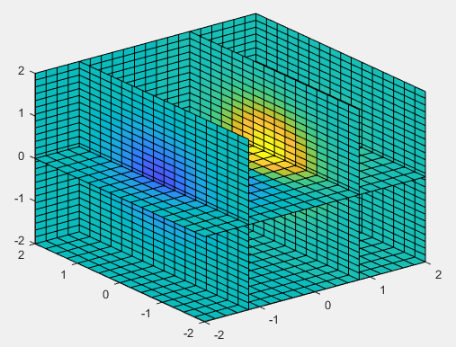
Example: Observe the volume situation of the function in the range -2≤x≤2, -2≤y≤2, -2≤z≤2.
% Data Preparation
xi=-10:0.5:10;
yi=-10:0.5:10;
[x,y]=meshgrid(xi,yi);
z=sin(sqrt(x.^2+y.^2))./sqrt(x.^2+y.^2);
[x,y,z] = meshgrid(-2:.2:2, -2:.25:2, -2:.16:2);
v = x.*exp(-x.^2-y.^2-z.^2);
xslice = [-1.2,.8,2];
yslice = 2;
zslice = [-2,0];
% Plotting
slice(x,y,z,v,xslice,yslice,zslice)
Copy
This concludes the article on MATLAB mathematical modeling and a summary of plotting techniques.