Click the image above to follow “Chuangxue Electronics” for easy learning of electronics knowledge.
This article does not encourage imitation; it merely shares the advanced functions of oscilloscopes. Similar methods include short-circuiting the ground line and signal pin of a passive probe to act as a near-field probe. Although the measurement results obtained from this method have errors, they provide a qualitative result without any cost.
The images in the article also show that this method, which has obvious errors, differs significantly from the measurement results obtained using a current probe.
PS: If you have the budget, do not skimp on a current probe and high-voltage differential probe. Measurement carries risks, and errors must be guarded against.
Problem Statement:
The oscilloscope is the most commonly used instrument by most electronic engineers. When mentioning oscilloscopes, people immediately think of voltage testing. Many oscilloscopes can also perform rough spectrum analysis, but many oscilloscopes cannot test a key indicator that electronic engineers care about—current. In some analysis and verification, not only is voltage testing required, but sometimes current testing is even more necessary. Currently, some high-end oscilloscopes can test current, but they require the purchase of active current probes, which can be quite expensive. The cost of purchasing an active current probe is comparable to that of some mid-range oscilloscopes, making it unaffordable for many small companies.
When it comes to current testing, some may ask if a multimeter can measure it. Indeed, a multimeter can measure current at a specific moment, but there are several issues: 1. Due to the slow response speed of multimeters (usually in the hundreds of milliseconds), trying to catch fleeting signals with such a response speed is like trying to chase a suspect on a high-speed train with a bicycle; 2. Multimeters cannot record long-term test results; some better models can record maximum and minimum values; 3. Most importantly, multimeters cannot show the process of current change. Many times, we want to see the process of change rather than just the result. For example, we want to know when a transistor is most likely to fail due to overcurrent, rather than just seeing it smoke.
Can we see the process of current change with an oscilloscope without an expensive current probe? Actually, we can find a solution by changing our thinking. The method is quite simple: we use Ohm’s Law, I=V/R. Note that this V is not the voltage at a single point but the potential difference between two points. This is key and is a common misconception for beginners. If you use the voltage change at a single point to infer the current change, you will often make mistakes, as we will see in the example tests below.
Specific Method:
The specific method is to measure the voltage V1 and V2 across a resistor (or even a segment of wire, provided that the resistance of this segment is large enough to create an appropriate potential difference across its ends). Then, using the oscilloscope’s calculation function, we can calculate △V=V1-V2 in real-time, and I=△V/R. As long as the environment does not undergo drastic changes, we can consider R to be constant, so I varies linearly with △V. Therefore, the change in △V reflects the change in current. We will verify whether this method is feasible through an example below.
Example Verification:
The oscilloscope screenshot below tests the voltage and current changes between the drain and source of an MOSFET at power-up. The brown waveform is the source voltage Vs, the purple waveform is the drain voltage Vd, and the yellow waveform is the calculated drain-source voltage △Vsd=Vs-Vd (in this example, channel C1 measures Vs, and channel C2 measures Vd, so the specific calculation setup is shown in Figure 2 as C1-C2). The green waveform is the drain-source current Isd measured with an active current probe. Comparing the waveforms of Isd and △Vsd, we can see that their change processes are very similar. The peak value of Isd measured with the active current probe is about 3.6A; the peak value of △Vsd calculated is about 0.43V. Using a multimeter, the resistance of this line is about 0.15Ω. Therefore, the current peak value obtained using the potential difference method is approximately 0.43V/0.15Ω = 2.87A. This differs from the result measured with the active current probe, of course, due to the different conduction resistances of the MOSFET in different states, the oscilloscope, passive probes, and the errors of the multimeter, etc. However, using this method to test the current change process we are most concerned with is entirely feasible. By observing the change in current, we can roughly know when the MOSFET is most likely to fail, thus providing a basis for taking the correct measures.
At this point, experienced engineers may raise a question: how to solve the common-mode rejection ratio (CMRR) when testing with ordinary probes? Indeed, this is a problem. However, we mentioned earlier that the main advantage of this method is that it allows us to see the change process of current. The accuracy of the specific current value tested using this method, influenced by various factors, is certainly not comparable to that of specialized active current probes (if this no-cost method could completely solve problems that cost tens of thousands, active current probes would no longer sell). Of course, if you happen to read this article and one day use the change in current to analyze and solve a past case, you might persuade your boss to skip a few drinks and buy a current probe instead. Moreover, to solve the CMRR, one would need to use an active differential probe, which is similarly expensive as a current probe, thus failing to meet our no-cost goal. However, the advantage of Vs-Vd is that it can eliminate some interference on the signal.
Additionally, we can see from the screenshot that the changes in the single-point voltages Vs or Vd differ from the changes in Isd, so do not fall into the trap of estimating current changes based on single-point voltage changes.
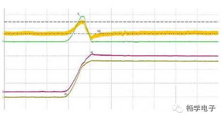
Figure 1: Obtaining the voltage difference by subtracting two voltages to approximate the measurement of current change.
Moreover, using this method requires that the oscilloscope has the data calculation function between channels (as shown in Figure 2). This function is a piece of cake for many oscilloscopes based on the Windows operating system. Of course, if the oscilloscope’s calculation formula can include R, i.e., the summary in Figure 2 as I=△V/R, the calculated results will be more intuitive.
Summary and Reflection:
There are always more methods than problems. In many cases, changing our perspective can lead to solutions. For example, many engineers are unable to observe the process of current change due to a lack of suitable instruments. They often rely on experience to estimate how current varies in a circuit, but such estimates may not match actual conditions. The method proposed in this article allows engineers to observe the process of current change in a circuit using existing oscilloscopes without spending money. Although its theoretical basis is not particularly sophisticated, it has good practical value, giving existing oscilloscopes an additional “eye.”
Actually, the idea for this article originated from my attempts years ago when my company had not yet purchased a current probe. At that time, I tried this approach because I lacked suitable tools but wanted to know how current varied. I hope to help many engineers in small and medium-sized companies who do not want to buy or cannot afford active current probes and are facing the same confusion I had back then.
> > > > > > > > > > > > > > > > > > > > > > > > > > > > > > > > > > > > > > > > > > > > > > > > > > > > > >
==> Visit www.eeskill.com to learn more!