
In digital circuit experiments, several instruments and meters are needed to observe experimental phenomena and results. Common electronic measuring instruments include multimeters, logic pens, ordinary oscilloscopes, storage oscilloscopes, logic analyzers, etc. The usage of multimeters and logic pens is relatively simple, while logic analyzers and storage oscilloscopes are not yet widely used in digital circuit teaching experiments. The oscilloscope is a widely used instrument that is relatively complex to operate. This chapter introduces the principles and usage methods of oscilloscopes from the user’s perspective.1. Working Principle of the Oscilloscope The oscilloscope utilizes the characteristics of the electron oscilloscope tube to convert alternating electrical signals that cannot be directly observed by the human eye into images displayed on a fluorescent screen for measurement. It is an essential instrument for observing phenomena in digital circuit experiments, analyzing problems during experiments, and measuring experimental results. The oscilloscope consists of an oscilloscope tube, power supply system, synchronization system, X-axis deflection system, Y-axis deflection system, delay scanning system, and standard signal source. 1.1. Oscilloscope Tube The cathode ray tube (CRT), referred to as the oscilloscope tube, is the core of the oscilloscope. It converts electrical signals into light signals. As shown in Figure 1, the electron gun, deflection system, and fluorescent screen are sealed within a vacuum glass shell, forming a complete oscilloscope tube.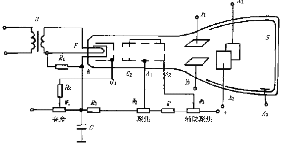 Figure 1 Internal Structure and Power Supply Diagram of the Oscilloscope Tube. The fluorescent screen of the current oscilloscope tube is usually a rectangular plane, with a layer of phosphorescent material deposited on the inner surface to form a phosphorescent film. An additional layer of evaporated aluminum film is often added on top of the phosphorescent film. High-speed electrons pass through the aluminum film, striking the phosphor to emit light and form bright spots. The aluminum film has a reflective effect, which helps enhance the brightness of the bright spots. The aluminum film also has other functions such as heat dissipation. When the electrons stop striking, the bright spot does not disappear immediately but retains for a period. The time taken for the brightness of the bright spot to decrease to 10% of its original value is called “afterglow time.” An afterglow time of less than 10μs is considered extremely short afterglow, 10μs to 1ms is short afterglow, 1ms to 0.1s is medium afterglow, 0.1s to 1s is long afterglow, and greater than 1s is extremely long afterglow. General oscilloscopes are equipped with medium afterglow tubes, high-frequency oscilloscopes select short afterglow, and low-frequency oscilloscopes select long afterglow. Due to the different phosphorescent materials used, different colors of light can be emitted from the fluorescent screen. Most general oscilloscopes use tubes that emit green light to protect human eyes. 2. Electron Gun and Focusing The electron gun consists of a filament (F), cathode (K), grid (G1), front accelerating electrode (G2) (also called the second grid), first anode (A1), and second anode (A2). Its function is to emit electrons and form a fine high-speed electron beam. The filament heats the cathode, causing it to emit electrons. The grid is a metal cylindrical tube with a small hole at the top, surrounding the cathode. Since the grid potential is lower than that of the cathode, it controls the electrons emitted by the cathode, allowing only a small number of electrons with high initial velocities to pass through the grid’s small hole under the influence of anode voltage and head towards the fluorescent screen. Electrons with lower initial velocities return to the cathode. If the grid potential is too low, all electrons return to the cathode, resulting in the tube being cut off. By adjusting the W1 potentiometer in the circuit, the grid potential can be changed to control the electron flow density directed towards the fluorescent screen, thereby adjusting the brightness of the bright spots. The first anode, second anode, and front accelerating electrode are three metal cylinders aligned with the cathode. The front accelerating electrode G2 is connected to A2, and its applied potential is higher than that of A1. The positive potential of G2 accelerates the electrons towards the fluorescent screen. During the journey from the cathode to the fluorescent screen, the electron beam undergoes two focusing processes. The first focusing is completed by K, G1, and G2, known as the first electron lens of the oscilloscope tube. The second focusing occurs in the G2, A1, and A2 region, where adjusting the voltage of the second anode A2 can cause the electron beam to converge precisely at a point on the fluorescent screen, which is the second focusing. The voltage on A1 is called the focusing voltage, and A1 is also referred to as the focusing electrode. Sometimes, even adjusting the A1 voltage does not achieve good focusing, requiring fine-tuning of the second anode A2’s voltage, which is also known as the auxiliary focusing electrode. 3. Deflection System The deflection system controls the direction of the electron beam, allowing the light spots on the fluorescent screen to depict the waveform of the measured signal as it changes with the applied signal. In Figure 8.1, the Y1, Y2, and X1, X2 pairs of mutually perpendicular deflection plates form the deflection system. The Y-axis deflection plates are in front, and the X-axis deflection plates are behind, making the Y-axis sensitivity higher (the measured signal is applied to the Y-axis after processing). The two pairs of deflection plates are each supplied with voltage, creating electric fields between them that control the deflection of the electron beam in both vertical and horizontal directions. 4. Power Supply for Oscilloscope Tubes To ensure that the oscilloscope tube operates normally, there are certain requirements for the power supply. The potential between the second anode and the deflection plates should be similar, and the average potential of the deflection plates should be zero or close to zero. The cathode must operate at a negative potential. The grid G1 is at a negative potential relative to the cathode (−30V to −100V) and is adjustable to achieve brightness adjustment. The first anode is at a positive potential (approximately +100V to +600V) and should also be adjustable for focusing adjustment. The second anode is connected to the front accelerating electrode, providing a positive high voltage (approximately +1000V) to the cathode, with an adjustable range relative to ground potential of ±50V. Since the currents of the electrodes in the oscilloscope tube are very small, a common high voltage can be supplied through a resistor divider. 1.2 Basic Components of the Oscilloscope As seen in the previous section, by controlling the voltages on the X-axis and Y-axis deflection plates, the shape of the displayed graph can be controlled. We know that an electronic signal is a function of time f(t) and varies with time. Therefore, by applying a voltage proportional to the time variable to the X-axis deflection plate and the measured signal (after proportional amplification or reduction) to the Y-axis, the oscilloscope screen will display the graph of the measured signal as it changes over time. In the electrical signal, a signal that is proportional to the time variable over a period is a sawtooth wave. The basic block diagram of the oscilloscope is shown in Figure 2. It consists of the oscilloscope tube, Y-axis system, X-axis system, Z-axis system, and power supply.
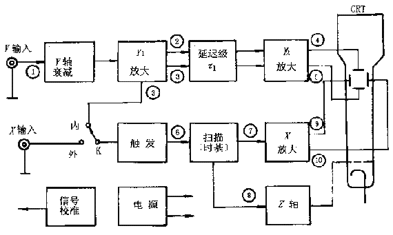 Figure 2 Basic Composition Block Diagram of the Oscilloscope. The measured signal ① is input to the “Y” input terminal, and after appropriate attenuation by the Y-axis attenuator, it is sent to the Y1 amplifier (pre-amplifier), producing push-pull output signals ② and ③. After a delay time Г1, it reaches the Y2 amplifier. After amplification, sufficiently large signals ④ and ⑤ are sent to the Y-axis deflection plate of the oscilloscope tube. To display a complete and stable waveform on the screen, the measured signal ③ from the Y-axis is introduced into the triggering circuit of the X-axis system, generating a trigger pulse ⑥ at a certain level of the positive (or negative) polarity of the introduced signal, which starts the sawtooth scanning circuit (time base generator), producing scanning voltage ⑦. Since there is a time delay Г2 from triggering to starting scanning, to ensure that the Y-axis signal reaches the fluorescent screen before the X-axis starts scanning, the delay time Г1 of the Y-axis should be slightly longer than the delay time Г2 of the X-axis. The scanning voltage ⑦ is amplified by the X-axis amplifier, producing push-pull outputs ⑨ and ⑩, which are sent to the X-axis deflection plate of the oscilloscope tube. The Z-axis system is used to amplify the positive scanning voltage and convert it into a positive rectangular wave, which is sent to the grid of the oscilloscope tube. This ensures that the waveform displayed during the positive scanning has a fixed brightness, while the scanning return process erases the trace. The above is the basic working principle of the oscilloscope. Dual trace display uses an electronic switch to separately display two different measured signals on the fluorescent screen. Due to the visual persistence of the human eye, when the switching frequency is high enough, two stable and clear signal waveforms are seen on the screen. There is often a precisely stable square wave signal generator in the oscilloscope for calibration purposes. 2. Using the Oscilloscope This section introduces the usage methods of the oscilloscope. There are many types and models of oscilloscopes, each with different functions. The most commonly used in digital circuit experiments are dual-trace oscilloscopes with 20MHz or 40MHz bandwidth. These oscilloscopes have similar usage methods. This section does not target a specific model of oscilloscope but introduces the commonly used functions of oscilloscopes in digital circuit experiments conceptually. 2.1 Fluorescent Screen The fluorescent screen is the display part of the oscilloscope tube. There are several scale lines in both horizontal and vertical directions on the screen, indicating the relationship between the voltage and time of the signal waveform. The horizontal direction indicates time, while the vertical direction indicates voltage. The horizontal direction is divided into 10 divisions, and the vertical direction is divided into 8 divisions, each further divided into 5 parts. The vertical direction is marked with 0%, 10%, 90%, 100%, etc., while the horizontal direction is marked with 10%, 90%, for measuring parameters such as DC level, AC signal amplitude, delay time, etc. By multiplying the number of divisions occupied by the measured signal on the screen by the appropriate proportional constant (V/DIV, TIME/DIV), the voltage and time values can be derived. 2.2 Oscilloscope Tube and Power Supply System 1. Power The main power switch of the oscilloscope. When this switch is pressed, the power indicator light turns on, indicating that the power is connected. 2. Brightness (Intensity) Turning this knob can change the brightness of the light spot and scanning line. When observing low-frequency signals, it can be lower, and for high-frequency signals, it can be higher. Generally, it should not be too bright to protect the fluorescent screen. 3. Focus The focus knob adjusts the size of the electron beam cross-section, focusing the scanning line into the clearest state. 4. Illuminance This knob adjusts the brightness of the lighting behind the fluorescent screen. In normal indoor lighting, it is better to keep the light dim. In poorly lit environments, it can be adjusted to be brighter. 2.3 Vertical Deflection Factor and Horizontal Deflection Factor 1. Vertical Deflection Factor Selection (VOLTS/DIV) and Fine Adjustment The distance the light spot moves on the screen under the action of a unit input signal is called the deflection sensitivity, which applies to both X-axis and Y-axis. The reciprocal of the sensitivity is called the deflection factor. The unit of vertical sensitivity is cm/V, cm/mV, or DIV/mV, DIV/V, while the unit of vertical deflection factor is V/cm, mV/cm, or V/DIV, mV/DIV. In practice, due to customary usage and the convenience of measuring voltage readings, the deflection factor is sometimes referred to as sensitivity. Each channel of the dual-trace oscilloscope has a vertical deflection factor selection band switch. Generally, the range is divided into 10 segments from 5mV/DIV to 5V/DIV in a 1, 2, 5 manner. The value indicated by the band switch represents the voltage value for one division in the vertical direction on the fluorescent screen. For example, when the band switch is set to the 1V/DIV range, if the signal light spot on the screen moves one division, it represents a change of 1V in the input signal voltage. Each band switch often also has a small knob for fine-tuning each vertical deflection factor. When it is turned clockwise to the end, it is in the “calibration” position, at which point the vertical deflection factor value is consistent with the value indicated by the band switch. Turning this knob counterclockwise allows for fine-tuning the vertical deflection factor. After fine-tuning the vertical deflection factor, it will result in a discrepancy from the value indicated by the band switch, which should be noted. Many oscilloscopes have a vertical expansion function, and when the fine-tuning knob is pulled out, the vertical sensitivity expands several times (the deflection factor decreases several times). For example, if the band switch indicates a deflection factor of 1V/DIV, in ×5 expansion mode, the vertical deflection factor is 0.2V/DIV. In digital circuit experiments, the ratio of the vertical movement distance of the measured signal on the screen to the vertical movement distance of a +5V signal is often used to determine the voltage value of the measured signal. 2. Time Base Selection (TIME/DIV) and Fine Adjustment The usage method for time base selection and fine adjustment is similar to that of vertical deflection factor selection and fine adjustment. The time base selection is also implemented through a band switch, dividing the time base into several segments in a 1, 2, 5 manner. The value indicated by the band switch represents the time value for the light spot to move one division in the horizontal direction. For example, in the 1μS/DIV range, moving the light spot one division on the screen represents a time value of 1μS. The “fine adjustment” knob is used for time base calibration and fine-tuning. When turned clockwise to the end, it is in the calibration position, where the displayed time base value on the screen is consistent with the nominal value indicated by the band switch. Rotating the knob counterclockwise allows for fine-tuning the time base. When the knob is pulled out, it is in the scanning expansion state, usually ×10 expansion, meaning the horizontal sensitivity is expanded by 10 times, and the time base is reduced to 1/10. For example, in the 2μS/DIV range, in scanning expansion mode, one division on the fluorescent screen represents a time value of 2μS × (1/10) = 0.2μS. The experimental platform has clock signals of 10MHz, 1MHz, 500kHz, and 100kHz generated by quartz crystal oscillators and frequency dividers, with high accuracy, which can be used to calibrate the oscilloscope’s time base. The oscilloscope’s standard signal source CAL is specifically used for calibrating the oscilloscope’s time base and vertical deflection factor. For example, the COS5041 model oscilloscope standard signal source provides a square wave signal with VP-P=2V, f=1kHz. The displacement (Position) knob on the front panel of the oscilloscope adjusts the position of the signal waveform on the fluorescent screen. Turning the horizontal displacement knob (marked with horizontal bidirectional arrows) moves the signal waveform left and right, while turning the vertical displacement knob (marked with vertical bidirectional arrows) moves the signal waveform up and down. 2.4 Input Channel and Input Coupling Selection 1. Input Channel Selection There are at least three ways to select the input channel: channel 1 (CH1), channel 2 (CH2), and dual channel (DUAL). When channel 1 is selected, the oscilloscope displays only the signal from channel 1. When channel 2 is selected, it displays only the signal from channel 2. When dual channel is selected, the oscilloscope displays both channel 1 and channel 2 signals simultaneously. When testing signals, the oscilloscope’s ground must first be connected to the ground of the circuit being tested. Depending on the input channel selection, the oscilloscope probe is plugged into the corresponding channel socket, connecting the ground of the oscilloscope probe with the ground of the circuit being tested, and the probe touches the test point. The oscilloscope probe has a dual-position switch. When this switch is set to the “×1” position, the measured signal is sent to the oscilloscope without attenuation, and the voltage value read from the fluorescent screen is the actual voltage value of the signal. When this switch is set to the “×10” position, the measured signal is attenuated to 1/10 before being sent to the oscilloscope, and the voltage value read from the fluorescent screen must be multiplied by 10 to obtain the actual voltage value of the signal. 2. Input Coupling Method There are three coupling methods: AC, ground (GND), and DC. When the ground option is selected, the scanning line shows the position of the “oscilloscope ground” on the fluorescent screen. DC coupling is used to determine the absolute value of the signal and observe very low-frequency signals. AC coupling is used to observe AC signals and AC signals containing DC components. In digital circuit experiments, the “DC” mode is generally selected to observe the absolute voltage value of the signal. 2.5 Triggering As mentioned in the first section, after the measured signal is input to the Y-axis, part of it is sent to the Y-axis deflection plate of the oscilloscope tube, driving the light spot to move vertically on the fluorescent screen proportionally; another part is diverted to the X-axis deflection system to generate a trigger pulse that triggers the scanning generator, producing a repetitive sawtooth voltage applied to the X deflection plate of the oscilloscope tube, causing the light spot to move horizontally. The combination of both results in the light spot depicting the graph of the measured signal on the fluorescent screen. Therefore, the correct triggering method directly affects the effective operation of the oscilloscope. To obtain a stable and clear signal waveform on the fluorescent screen, mastering the basic triggering functions and their operation methods is very important. 1. Trigger Source Selection To display a stable waveform on the screen, the measured signal itself or a trigger signal with a certain time relationship to the measured signal must be applied to the triggering circuit. The trigger source selection determines where the trigger signal is supplied from. There are usually three trigger sources: internal trigger (INT), line trigger (LINE), and external trigger (EXT). Internal trigger uses the measured signal as the trigger signal and is a commonly used method. Since the trigger signal itself is part of the measured signal, a very stable waveform can be displayed on the screen. In dual-trace oscilloscopes, either channel 1 or channel 2 can be selected as the trigger signal. Line trigger uses the AC mains frequency signal as the trigger signal. This method is effective when measuring signals related to AC mains frequency, especially when measuring audio circuits or low-level AC noise from thyristors. External trigger uses an external signal as the trigger signal, which is input from the external trigger input terminal. The external trigger signal should have a periodic relationship with the measured signal. Since the measured signal is not used as the trigger signal, when scanning starts is independent of the measured signal. Correctly selecting the trigger signal greatly influences the stability and clarity of the waveform display. For example, in digital circuit measurements, for a simple periodic signal, internal triggering might be better, while for a complex periodic signal with a periodic relationship with another signal, external triggering may be preferable. 2. Trigger Coupling Method The coupling method for the trigger signal to the triggering circuit varies, with the goal of ensuring the stability and reliability of the trigger signal. Here are some commonly used methods. AC coupling, also known as capacitive coupling, allows only the AC component of the trigger signal to pass through while blocking the DC component. This method is typically used when the DC component is not considered, to achieve stable triggering. However, if the trigger signal frequency is less than 10Hz, it can cause triggering difficulties. DC coupling does not block the DC component of the trigger signal. When the trigger signal frequency is low or its duty cycle is large, DC coupling is preferable. Low-frequency suppression (LFR) triggering applies a high-pass filter to the trigger signal before it reaches the triggering circuit, suppressing the low-frequency components of the trigger signal; high-frequency suppression (HFR) triggering applies a low-pass filter, suppressing the high-frequency components. There are also TV sync (TV) triggering methods used for television repairs. Each of these coupling methods has its own applicable range and should be experienced during use. 3. Trigger Level and Trigger Polarity Trigger level adjustment, also known as synchronization adjustment, synchronizes the scanning with the measured signal. The level adjustment knob adjusts the trigger level of the trigger signal. Once the trigger signal exceeds the level set by the knob, scanning is triggered. Turning the knob clockwise raises the trigger level; counterclockwise lowers it. When the level knob is set to the level lock position, the trigger level automatically remains within the amplitude of the trigger signal without requiring further adjustment. When the signal waveform is complex and cannot be stabilized with the level knob, the hold-off knob can be adjusted to manage the hold-off time (scan pause time) of the waveform, allowing synchronization with the waveform. The polarity switch is used to select the polarity of the trigger signal. When set to the “+” position, it triggers when the signal increases past the trigger level; when set to the “-” position, it triggers when the signal decreases past the trigger level. The trigger polarity and trigger level together determine the trigger point of the trigger signal. 2.6 Scanning Mode There are three scanning modes: automatic (Auto), normal (Norm), and single (Single). Automatic: When no trigger signal is input or the trigger signal frequency is below 50Hz, scanning is self-oscillating. Normal: When no trigger signal is input, scanning is in a ready state, with no scanning line. When the trigger signal arrives, scanning is triggered. Single: The single button is similar to a reset switch. In single scanning mode, pressing the single button resets the scanning circuit, and the ready light turns on. When the trigger signal arrives, a single scan is produced. After the single scan ends, the ready light goes out. Single scanning is used to observe non-periodic signals or single transient signals, often requiring waveform capture. The above briefly introduces the basic functions and operations of oscilloscopes. Oscilloscopes also have more complex functions, such as delayed scanning, trigger delay, and X-Y operation modes, which are not covered here. The basic operation of oscilloscopes is easy, but true proficiency requires mastery through application. It is worth noting that although oscilloscopes have many functions, in many cases, other instruments may perform better. For instance, in digital circuit experiments, using a logic pen is much simpler for determining whether a narrow pulse has occurred, while a logic analyzer is better for measuring pulse width. Issues to Note When Using Digital Oscilloscopes Introduction Digital oscilloscopes are increasingly popular due to their unique advantages in waveform triggering, storage, display, measurement, and waveform data analysis. However, there are significant performance differences between digital and analog oscilloscopes, and improper use can lead to considerable measurement errors, affecting testing tasks. Distinguishing Between Analog Bandwidth and Digital Real-Time Bandwidth Bandwidth is one of the most important indicators of an oscilloscope. The bandwidth of an analog oscilloscope is a fixed value, while the digital oscilloscope has both analog bandwidth and digital real-time bandwidth. The highest bandwidth achievable by a digital oscilloscope for repetitive signals using sequential sampling or random sampling techniques is its digital real-time bandwidth, which is related to the maximum digital frequency and waveform reconstruction factor K (digital real-time bandwidth = maximum digitization rate/K). This is generally not presented as a direct indicator. From the definitions of the two types of bandwidth, it can be seen that analog bandwidth is only suitable for measuring repetitive periodic signals, while digital real-time bandwidth is suitable for measuring both repetitive and single-shot signals. Manufacturers often state the bandwidth of an oscilloscope in megahertz, which actually refers to the analog bandwidth, while the digital real-time bandwidth is lower than this value. For example, TEK’s TES520B has a bandwidth of 500MHz, which refers to its analog bandwidth of 500MHz, while the highest digital real-time bandwidth can only reach 400MHz, significantly lower than the analog bandwidth. Therefore, when measuring single-shot signals, it is essential to refer to the digital oscilloscope’s digital real-time bandwidth; otherwise, unexpected measurement errors may occur. About Sampling Rate The sampling rate, also known as digitization rate, refers to the number of samples taken per unit time of the analog input signal, commonly expressed in MS/s. The sampling rate is an important indicator of digital oscilloscopes. 1. If the sampling rate is insufficient, aliasing can easily occur. For instance, if the input signal to the oscilloscope is a 100KHz sine wave, but the displayed signal frequency is 50KHz, this is due to the oscilloscope’s sampling rate being too slow, resulting in aliasing. Aliasing occurs when the frequency displayed on the screen is lower than the actual signal frequency, or even when the trigger indicator on the oscilloscope is lit, the displayed waveform remains unstable. The occurrence of aliasing is illustrated in Figure 1. So, how can one determine whether the displayed waveform has already experienced aliasing for an unknown frequency waveform? One can slowly change the sweep speed t/div to a faster time base setting and observe whether the frequency parameter of the waveform changes dramatically; if so, aliasing has occurred. Alternatively, if a wavering waveform stabilizes at a certain faster time base setting, it also indicates that aliasing has occurred. According to the Nyquist theorem, the sampling rate must be at least twice the highest frequency component of the signal to avoid aliasing. For a 500MHz signal, a sampling rate of at least 1GS/s is required. Here are several methods to simply prevent aliasing from occurring: • Adjust the sweep speed; • Use the auto set (Autoset) function; • Try switching the collection method to envelope mode or peak detection mode, as envelope mode seeks extremes in multiple collection records, while peak detection mode finds maximum and minimum values in a single collection record; both methods can detect rapid signal changes. • If the oscilloscope has an InstaVu collection mode, it can be selected, as this mode captures waveforms quickly, producing a display similar to that of an analog oscilloscope. 2. The Relationship Between Sampling Rate and t/div Each digital oscilloscope has a maximum sampling rate, which is a constant value. However, for any given sweep time t/div, the sampling rate fs is given by the formula: fs = N/(t/div), where N is the number of sampling points per division. When the number of sampling points N is a constant value, fs is inversely proportional to t/div; the faster the sweep speed, the lower the sampling rate. Below is a set of data from the TDS520B showing the relationship between sweep speed and sampling rate:
| t/div (ns) | fs (GS/s) |
|---|---|
| 125 | 50 |
| 255 | 25 |
| 1000 | 10 |
| 2000 | 0.5 |
In summary, when using a digital oscilloscope, to avoid aliasing, it is best to set the sweep speed to a faster setting. If you want to capture fleeting glitches, it is preferable to set the sweep speed to a slower main sweep setting.
The rise time of digital oscilloscopes is extremely important. In analog oscilloscopes, rise time is a crucial indicator. However, in digital oscilloscopes, rise time is not even clearly specified as an indicator. Due to the measurement methods of digital oscilloscopes, the automatically measured rise time is not only related to the position of the sampling points, as shown in Figure 2. In case a rise edge falls exactly between two sampling points, the rise time is 0.8 times the digitization interval. In case the rise edge’s center is at a sampling point, the same waveform results in a rise time of 1.6 times the digitization interval. Furthermore, rise time is also related to sweep speed. Below is a set of data from the TDS520B measuring the same waveform showing the relationship between sweep speed and rise time:
| t/div (ms) | tr (μs) |
|---|---|
| 50 | 8 |
| 20 | 3.2 |
| 10 | 1.6 |
| 5 | 0.8 |
From this data, it can be seen that although the rise time of the waveform is a constant value, the results measured with a digital oscilloscope can vary greatly depending on the sweep speed. The rise time of an analog oscilloscope is independent of sweep speed, while the rise time of a digital oscilloscope is not only affected by sweep speed but also by the position of the sampling points. When using a digital oscilloscope, we cannot deduce the rise time of the signal based on the measured time as we would with an analog oscilloscope.
(Source: Mastering Microcontrollers)

This issue was edited by: QQ
Editor: Electronics Department Student Union Media Office

