“The FFT function on an oscilloscope is a tool that provides a frequency domain view of signals. Understanding how the FFT function on the oscilloscope can bring digital and RF designs to market.”
How to Access FFT on Keysight Oscilloscopes
Why Are There Different Window Options for FFT?
The video below also demonstrates how to use Keysight’s FFT testing:
Basic Principles of FFT Spectrum Analysis on Oscilloscopes
Several factors can affect the accuracy and precision of FFT spectrum analysis on oscilloscopes. These factors will be discussed below.
We must understand how the sampling characteristics of the oscilloscope impact the quality of FFT testing. The analog bandwidth, sampling rate, memory depth, and capture time of the oscilloscope profoundly affect the measurement results, and this influence also depends on the characteristics of the measured signal and the relationship between those signal characteristics and the oscilloscope’s capture performance.
For example, in this simple example, we want to measure a single-tone 600 MHz sine wave signal and observe the basic spectral characteristics of this signal. The oscilloscope must have sufficient analog bandwidth to avoid attenuation of the signal’s amplitude. Since this oscilloscope has a maximum analog bandwidth of 1 GHz, it is sufficient to measure a 600 MHz audio signal. This measurement will demonstrate that the time/scale settings are crucial for maintaining this bandwidth during measurement.
To avoid aliasing during the digitization of the signal, the sampling speed must be at least twice that of any perceivable frequency in the measured signal. In this simplest sine wave example, measuring this 600 MHz sine wave requires a sampling rate of at least 1.2 GHz. Clearly, this oscilloscope’s maximum sampling rate of 5 GSa/s is more than sufficient for this measurement. However, to achieve at least a 1.2 GHz sampling rate, the oscilloscope’s time/scale settings must be maintained within a specific range.
What quality can we expect from the FFT test of this 600 MHz sine wave? Let’s return to the FFT measurement in Figure 1. Note the prominent single-frequency peak, with the corresponding measurement cursor indicating a frequency of about 600 MHz and a power of 0 dBm, which aligns with expectations.
The spacing between actual spectral lines driven by the FFT data is known as “resolution bandwidth.” Due to the distribution of signal energy, this is sometimes referred to as frequency “bin” width. The resolution bandwidth is strictly based on the time length of the acquired data and the type of FFT window selected. Here, a rectangular window is used, with a factor of “1,” so the resolution bandwidth is the inverse of the recording time. In this case:
Resolution Bandwidth = 1 / (200 ns/scale x 10 scales) = 500 kHz
Therefore, this FFT can distinguish frequency components in the signal spectrum that are spaced more than 500 kHz apart, while frequency components spaced less than 500 kHz will blend together and become indistinguishable. The FFT “resolution bandwidth” should not be confused with the “FFT resolution” number displayed on the screen (153 kHz). The latter describes the actual spacing between two FFT points in the FFT data but does not represent the actual resolution bandwidth obtained over the specified time span.
How Time/Scale Reduction Affects Oscilloscope FFT Response Performance
To demonstrate the importance of recording time on FFT results, if the time/scale is magnified to 1 ns/scale, showing only 10 ns of new time records on the screen, the resolution bandwidth will rapidly change to:
Resolution Bandwidth = 1 / (10 ns) = 100 MHz
The significant change in FFT results is shown in Figure 2, where the 600 MHz frequency domain peak is displayed more coarsely. A trade-off has occurred here. The less time sampling is processed, the fewer spectral lines calculated in the FFT results, leading to poorer resolution bandwidth, but the speed of the FFT test has greatly increased.
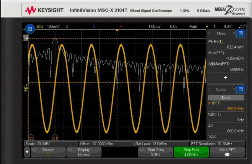
Figure 2. Time-domain capture results with a 600 MHz sine wave input and FFT calculation at 1 ns/scale.
Considerations for Time/Scale Settings
If the time/scale settings are set too small, it results in too short a time record displayed on the screen, with too few time points, reducing the performance of the FFT test (as shown previously). Conversely, if the time/scale settings are too large, causing the time record displayed on the screen to be too long, it can also cause issues, as the oscilloscope will reduce the sampling rate to maintain good throughput.
For example, the time/scale setting can be adjusted upward to 200 ns/scale, displaying a 2 μs time record on the screen, under which conditions the oscilloscope can maintain a sampling rate of 5 Gsa/s and an analog bandwidth of 1 GHz. However, at settings of 330 ns/scale and higher, the sampling rate decreases, and the oscilloscope’s bandwidth reduces, affecting the FFT results.
Using Start Frequency, Stop Frequency, Center Frequency, and Sweep Width Control
An important feature of FFT calculations and result views is the ability to zoom in on the area of interest. The first example has a wide frequency sweep from 0 Hz to 2.5 GHz, making it difficult to see any details near the 600 MHz carrier. If there is suspicious noise near the 600 MHz carrier frequency and you want to check this noise, the FFT control function can set the center frequency to 600 MHz and establish a target sweep width, for example, 100 MHz around the 600 MHz carrier. Setting a start frequency of 550 MHz and a stop frequency of 650 MHz will also yield the same result. The FFT test with these parameters is shown in Figure 3.
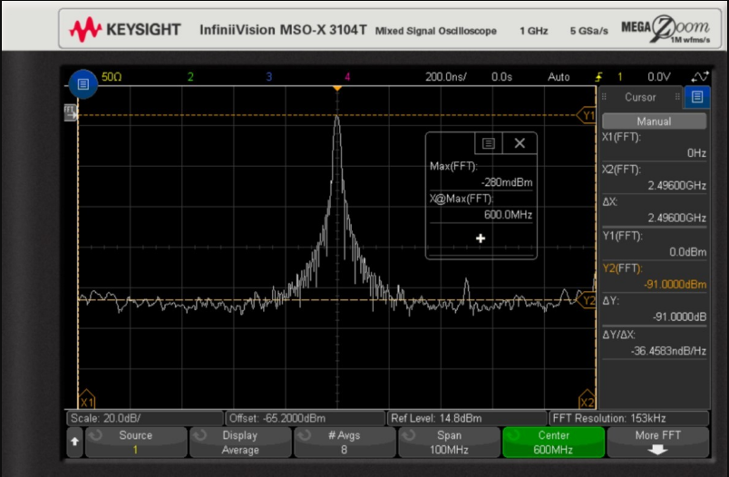
Figure 3. FFT results for a 600 MHz sine wave input, with FFT control set to a center frequency of 600 MHz and a sweep width of 100 MHz.
Wideband FFT Analysis
Nowadays, more and more signals are modulated, which can increase the spectrum width to hundreds of MHz or even several GHz. If the bandwidth of the signal exceeds 510 MHz, current spectrum analyzers or vector signal analyzers on the market do not have sufficient analysis bandwidth for effective measurement. In this case, an oscilloscope or digitizer with sufficient wide analysis bandwidth is required to meet application needs. The carrier frequency of the measured signal is also important. The carrier frequency of the signal plus half of the signal’s spectrum width must be less than or equal to the bandwidth of the oscilloscope for it to perform the measurement independently.
Now we will discuss wideband signal frequency domain measurements. The measured signal is a 600 MHz RF pulse train, repeating every 20 μs with 4 μs wide RF pulses. We perform a 600 MHz linear frequency modulation on this signal, meaning linear frequency modulation of the RF pulse envelope from 300 MHz to 900 MHz.
To conduct the basic FFT test of the RF pulse, the first step is to capture a clean time-domain pulse on the screen. Use trigger hold-off to ensure that the trigger does not occur in the middle of the pulse, avoiding unstable traces in the captured waveform. The trigger hold-off is set to slightly longer than the width of the RF pulse. Since the RF pulse is 4 μs wide, the trigger hold-off can be set to 5 μs.
The simplest way to define the trigger hold-off is to press the “Mode/Coupling” button in the trigger area on the front panel and then select a 5 μs trigger hold-off time.
Then press the “FFT” button to calculate the frequency spectrum view of the RF pulse train from the time-domain digitized signal on the screen. The oscilloscope provides FFT control functions such as start and stop frequency or center frequency and sweep width. First, select a wider sweep width with a start frequency of 0 Hz and a stop frequency of 2.5 GHz. Choose a rectangular window for the FFT calculation, as the data on the screen starts and ends with noise, and the entire RF pulse is within the screen window. Performing 8 FFT averages also helps optimize measurement results. Figure 4 shows the FFT response results.
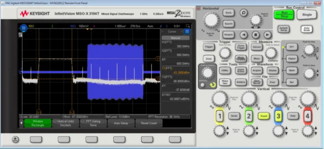
Figure 4. FFT results for a 4 μs pulse width and 20 μs repetition period linear frequency-modulated pulse signal.
The cursor placed on the FFT response shows that this RF pulse has a frequency spectrum width of 600 MHz, ranging from 300 MHz to 900 MHz. It has not yet been proven that the carrier frequency linearly transitions from 300 MHz to 900 MHz, spanning from the left side of the pulse to the right side of the pulse.
Gated FFT Calculation Function
To quickly see certain carrier frequency values on the pulse, one method is to use the gated FFT function. This can be achieved by activating the normal time-domain trace gating function.Once activated, the upper half of the screen will display a normal trace view, while the lower half will show an enlarged view. Any part of the waveform that appears in the lower trace window is magnified.
By creating a small time-width window function and then moving it to the start of the pulse, we can obtain the measurement results we are interested in. The FFT can be calculated using the data contained in the time gating window shown in Figure 5.
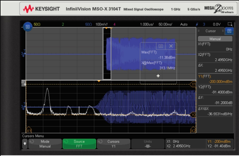
Figure 5. Time gating FFT function observing the carrier at the start of the RF pulse.
The FFT measurement results for peak amplitude and frequency show that the RF pulse starts at a carrier frequency of about 300 MHz. If the time gating window is moved to the center of the RF pulse, the observed frequency is around 600 MHz. At the end of the RF pulse, it is 900 MHz. This appears to be the expected linear frequency modulation.
Frequency Measurements and Measurement Trend Function
In some cases, the “Measurement Trend” function can effectively display the frequency linear frequency modulation curve.In a similar signal example, a pulse train consists of RF pulses that are 700 ns wide, repeating every 20 μs.We need to verify its linear frequency modulation characteristics between 300 MHz and 900 MHz.With the FFT function now turned off, we conduct pure time-domain measurements.
First, switch the oscilloscope’s acquisition mode from “Normal” to “High Resolution” mode. Secondly, select a frequency measurement from the candidate measurement list. The mid-threshold for zero-crossing detection of the carrier is set to 30 mV. Then press the “Math” button and select the “Measurement Trend” function. The marked results are the outcomes of the calculations. The frequency measurement results across the RF pulse are shown in Figure 6.
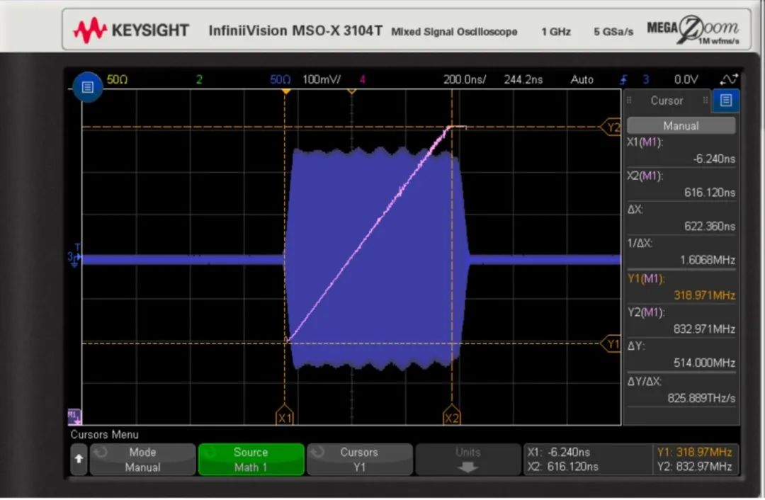
Figure 6. Measurement trend function of frequency measurement across pulses.
Clearly, the pulse carrier moves linearly from left to right across the entire pulse as designed. The vertical cursor shows that the starting frequency begins at about 320 MHz, ending at around 830 MHz, with the horizontal cursor indicating that this event lasts approximately 600 ns. Thus, the calculated linear frequency modulation slope is 0.85 MHz/ns. The expected linear frequency modulation slope would move 600 MHz over a 700 ns wide pulse (including the rise and fall times of the envelope), or 0.86 MHz/ns. The measured linear frequency modulation slope matches the expectation.
Note that the linear slope display does not span the entire width of the RF pulse but reaches a limit before the end of the pulse. This is because the measurement limit of 1000 has been reached in the trend calculations. Importantly, we can see that part of the pulse’s FM function is linear. To achieve sufficient accuracy for frequency measurements across the pulse, the “High Resolution” acquisition mode must be selected.
To select the “High Resolution” mode, press the “Acquire” button in the waveform area on the front panel and then choose “High Resolution”.
If the carrier crosses the pulse at higher frequency ranges, such as double the aforementioned range (900 MHz to 1.8 GHz), the linear slope can only be observed over half the pulse width. For applications in higher frequency ranges, such as general radar systems, the Infiniium S series, V series, or Z series oscilloscopes can be selected, as their measurement trend functions do not have the 1000 measurement limit.
Simple Example of FFT Testing with Input Sine Wave
The MSO-X 3104T mixed signal oscilloscope has a 1 GHz analog bandwidth and a sampling rate of up to 5 GSa/s, capable of performing various measurements.These two technical specifications are critical and directly relate to which measurement applications can be achieved.The first measurement example we discussed is capturing a 600 MHz, 632 mV (peak-to-peak), 0 dBm, 1 mW sine wave signal injected into a 50 Ω resistor (orange), along with the FFT results (white), as shown in Figure 1.
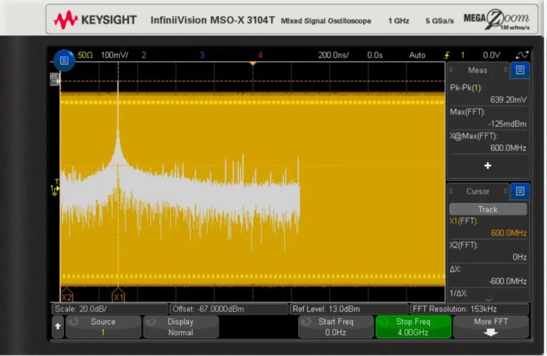
Figure 1. Time-domain capture and FFT calculation results using a 600 MHz sine wave input at 200 ns/scale.
Conclusion
FFT spectrum analysis on oscilloscopes is a valuable tool that provides a frequency domain view of signals, allowing oscilloscopes to perform measurements over a very wide bandwidth, completing measurements that narrowband vector signal analyzers cannot. Examples of oscilloscope FFT tests can validate whether linear FM modulated signals move the carrier frequency as intended. Additionally, oscilloscopes offer other operational features, including the measurement trend function.
Disclaimer:
For submissions/recruitment/promotion/advertising, please add WeChat: 15989459034