★
Embedded AI Series – Analysis of YOLOv5 Model Deployment Example Code on RK RV1126 Platform – 2 Memory Distribution of Model Outputs
”
1. Introduction
- The remaining important part of the source code in rknn_yolov5_demo is the post-processing.
- The post-processing of the official YOLOv5 model is included within the model, so no post-processing is required for the official model output. However, due to hardware limitations of the RK platform, the post-processing module has been removed from the rknn format YOLOv5 model, and instead, the processing is handled in the CPU using code, which is concentrated in the function post_process.
2. Original Output Format and Memory Distribution of the Model
To parse the model’s output in the post-processing function, it is necessary to first understand the output format and memory distribution of the model.
The article “Embedded AI Series – Analysis of YOLOv3 Deployment Code on RV1126 – Post-processing 1” provides a detailed explanation of the original output format, memory distribution, and some related concepts of the YOLOv3 model, which can be referenced for reading.
The output of YOLOv5 is quite similar to that of YOLOv3, with the following similarities:
1. Outputs three tensor grid feature maps, used for detecting small, medium, and large targets;
2. Each grid within the feature map contains predictions for three prior anchor boxes;
3. For the COCO dataset with 80 classes, the prediction results for each prior box contain 4 (4 coordinate values) + 1 (1 confidence score) + 80 (80 class conditional probabilities) = 85 values;
4. Thus, the number of channels C for each output layer tensor is C = 3 * (5 + 80) = 255. Each grid corresponds to 255 values, so for a 20 * 20 grid feature map, the output memory size is: 20 * 20 * 255 = 102000 bytes;
The differences between the outputs of YOLOv5 and YOLOv3 are:
1. The sizes of the three feature maps are different;
2. The formulas used for decoding bounding box coordinates are different: YOLOv5 has made an improvement in the calculation of the center point coordinates by introducing an offset strategy;
3. The meanings of object confidence and class probability are different: YOLOv5 combines the predictions of object confidence and class probability.
2.1 Original Output Format of the Model
The description of the similarities above focuses on the format of the data for each grid in the feature map, continuing with a previous diagram for illustration:
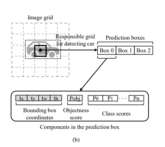
Image source:
https://openaccess.thecvf.com/content_ICCV_2019/papers/Choi_Gaussian_YOLOv3_An_Accurate_and_Fast_Object_Detector_Using_Localization_ICCV_2019_paper.pdf
In the above image, “Image grid” represents a feature map, where each grid contains the contents of three prior boxes (Prediction boxes). Each prior box contains 4 box coordinates plus 1 object confidence score, followed by 80 class conditional probabilities; thus, each grid corresponds to 3 * (5 + 80) = 255 values, which is the meaning of the channels in the model output format.
For the output of the YOLOv5 model in this example, the printed results from running the program are as follows:

As can be seen, the output of YOLOv5 has three tensors:
- The size of the first output tensor feature map is 80 * 80, with each grid having 255 channels, resulting in a memory size of 80 * 80 * 255 = 1632000 bytes;
- The size of the second output tensor feature map is 40 * 40, with each grid having 255 channels, resulting in a memory size of 40 * 40 * 255 = 408000 bytes;
- The size of the third output tensor feature map is 20 * 20, with each grid having 255 channels, resulting in a memory size of 20 * 20 * 255 = 102000 bytes;
2.2 Memory Distribution of Model Output Cache
The three output tensors of the YOLOv5 model are each saved using a data type of rknn_output, where the member variable buf of rknn_output is assigned to save the pointer to the cache buffer of each tensor feature map data. The post-processing function post_process in the demo code parses the memory pointed to by rknn_output->buf to obtain the detection results.
Taking the 20 x 20 feature map as an example, a detailed breakdown of the original output memory distribution of the YOLOv5 model before post-processing is as follows:
This segment 13202085 = 102,000 data points are arranged in memory in a continuous linear fashion. The order can be imagined as an “onion”, unfolding layer by layer from the outside:
Outermost layer: Batch (size 1, can be ignored)
Second layer: Anchor index (a) → First arrange all data for the first anchor box (a=0), then the second anchor box (a=1), and finally the third anchor box (a=2).
Third layer: Grid Y coordinate (gy) → For a fixed anchor box, traverse the grid row by row. First arrange all data for gy=0, then gy=1, …, and finally gy=19.
Fourth layer: Grid X coordinate (gx) → For a fixed gy, traverse the grid column by column. First arrange the data for gx=0, then gx=1, …, and finally gx=19.
Innermost layer: Attributes (attr) → For a fixed grid point (gy, gx) and a fixed anchor box (a), tightly arrange its 85 attribute values, strictly following the order [t_x, t_y, t_w, t_h, o, cls1, cls2, …, cls80].
| Memory Address Offset Range | Corresponding Dimension Index | Meaning |
|---|---|---|
| 0 ~ 84 | [0, 0, 0, 0, :] | 85 attribute values for the first anchor box (a=0), first grid (gy=0, gx=0). |
| 85 ~ 169 | [0, 0, 0, 1, :] | 85 attribute values for the first anchor box (a=0), second grid (gy=0, gx=1). |
| … | … | … (continue traversing gx=2 to gx=19) |
| 1700 ~ 1784 | [0, 0, 1, 0, :] | 85 attribute values for the first anchor box (a=0), second row (gy=1), first column (gx=0) grid. |
| … | … | …(continue traversing all 20×20=400 grid points for the first anchor box) |
| 33,915 ~ 33,999 | [0, 0, 19, 19, :] | 85 attribute values for the first anchor box (a=0), last row (gy=19), last column (gx=19) grid. |
| 34,000 ~ 34,084 | [0, 1, 0, 0, :] | 85 attribute values for the second anchor box (a=1), first grid (gy=0, gx=0). |
| 34,085 ~ 34,169 | [0, 1, 0, 1, :] | 85 attribute values for the second anchor box (a=1), second grid (gy=0, gx=1). |
| … | … | …(start repeating the entire process, but for the second anchor box) |
| 68,000 ~ 68,084 | [0, 2, 0, 0, :] | 85 attribute values for the third anchor box (a=2), first grid (gy=0, gx=0). |
| … | … | … (continue traversing until the end) |
| 101,915 ~ 101,999 | [0, 2, 19, 19, :] | 85 attribute values for the third anchor box (a=2), last row (gy=19), last column (gx=19) grid. |
This method is similar to the RGB format of Packed / Interleaved Format.
2.3 Memory Distribution of rknn Model Output Cache
However, unlike the conventional YOLOv5 model output memory distribution described in section 2.2, the pre-compiled rknn model used in rknn_yolov5_demo employs a mixed memory arrangement: interleaved prior boxes + planar format within boxes:
- 1. Between prior boxes: arranged in order (Anchor 0 → Anchor 1 → Anchor 2)
- 2. Within prior boxes: arranged in planar format (all grid points of the same attribute are stored continuously)
Taking the 20 x 20 feature map as an example, the original output memory distribution of the rknn format YOLOv5 model before post-processing is as follows:
1. Anchor 0 Block (Offset: 0 – 33,999)
// Attribute 0: t_x (all grid points) address 0: t_x address of grid(0,0) 1: t_x address of grid(0,1)... address 19: t_x address of grid(0,19) 20: t_x address of grid(1,0)... address 399: t_x address of grid(19,19)// Attribute 1: t_y (all grid points) address 400: t_y address of grid(0,0) 401: t_y address of grid(0,1)... address 799: t_y address of grid(19,19)// Attribute 2: t_w (all grid points) address 800: t_w address of grid(0,0) 801: t_w address of grid(0,1)... address 1199: t_w address of grid(19,19)// Attribute 3: t_h (all grid points) address 1200: t_h address of grid(0,0) 1201: t_h address of grid(0,1)... address 1599: t_h address of grid(19,19)// Attribute 4: Object confidence (all grid points) address 1600: Object confidence address of grid(0,0) 1601: Object confidence address of grid(0,1)... address 1999: Object confidence address of grid(19,19)// Attribute 5-84: Class confidence (all grid points) address 2000: Class 0 confidence address of grid(0,0) 2001: Class 0 confidence address of grid(0,1)... address 2399: Class 0 confidence address of grid(19,19) address 2400: Class 1 confidence address of grid(0,0) 2401: Class 1 confidence address of grid(0,1)... address 2799: Class 1 confidence address of grid(19,19)... address 33600: Class 79 confidence address of grid(0,0) 33601: Class 79 confidence address of grid(0,1)... address 33999: Class 79 confidence address of grid(19,19)2. Anchor 1 Block (Offset: 34,000 – 67,999)
// Structure same as Anchor 0, but corresponding to the second prior box address 34000: t_x address of grid(0,0) (Anchor 1) address 34001: t_x address of grid(0,1) (Anchor 1)... address 67999: Class 79 confidence address (Anchor 1)3. Anchor 2 Block (Offset: 68,000 – 101,999)
// Structure same as Anchor 0, but corresponding to the third prior box address 68000: t_x address of grid(0,0) (Anchor 2) address 68001: t_x address of grid(0,1) (Anchor 2)... address 101999: Class 79 confidence address (Anchor 2)To access the value of a specific prior box, specific attribute, and specific grid position, refer to the following formula in the Python code:
def get_value(data, anchor_idx, attribute_idx, row, col): # Size of each Anchor block: 85 attributes × 400 grid points = 34,000 anchor_offset = anchor_idx * 34000 # Size of each attribute plane: 20 rows × 20 columns = 400 attribute_offset = attribute_idx * 400 # Grid offset: row * 20 + col grid_offset = row * 20 + col # Total offset total_offset = anchor_offset + attribute_offset + grid_offset return data[total_offset]In the post-processing function process of the rknn_yolov5_demo source code, this formula is used to retrieve the required attribute values:
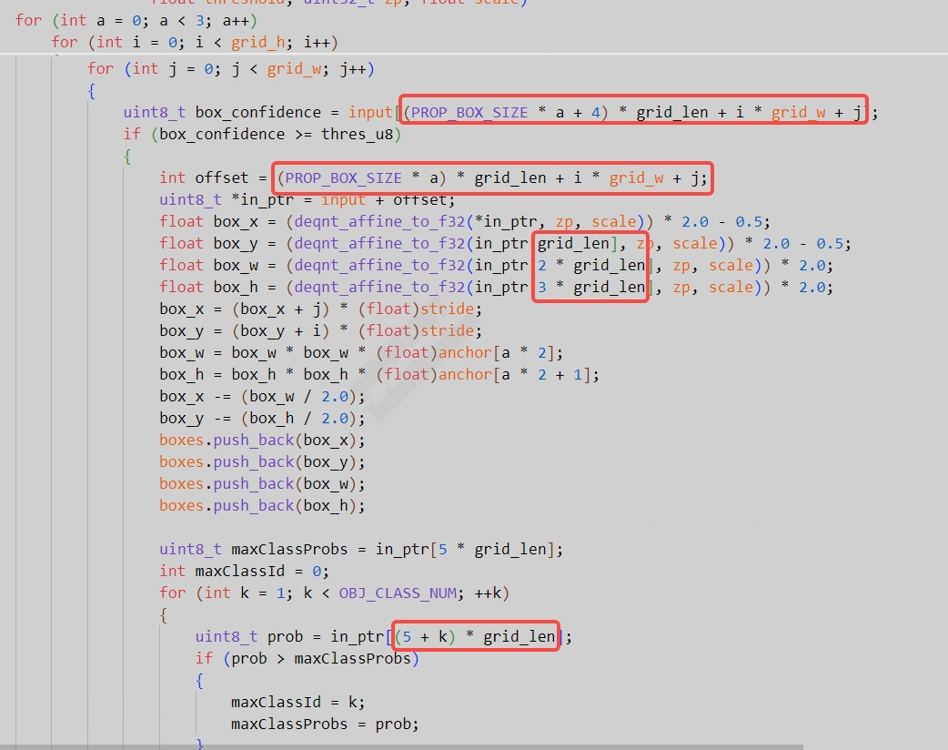
This mixed arrangement method balances the needs of data access patterns and computational efficiency, which is particularly useful in embedded devices and dedicated hardware accelerators.
Understanding the memory arrangement of the rknn model output is crucial for comprehending the post-processing part of the source code.
Other functions in the post-processing function, such as NMS, can be referenced in the article “Embedded AI Series – Analysis of YOLOv3 Deployment Code on RV1126 – Post-processing 3” and will not be elaborated on here.