In electronic circuit design, the Bode plot is an essential tool for analyzing the frequency characteristics of circuits. However, professional instruments often start at a high price, making them unfriendly for beginners and makers. Today, we present a low-cost, easy-to-use open-source project— based on the STM32G031 microcontroller, which accurately collects analog signals through ADC and uses a Python host computer to plot amplitude and phase frequency response curves in real-time, achieving Bode plot measurements at a hardware cost of around a hundred yuan! Whether it’s developing STM32 peripherals, optimizing ADC timing, or applying FFT algorithms in frequency domain analysis, this project helps us deeply master the core technologies of embedded systems and signal processing in practice.The project has been open-sourced on EETREE: https://www.eetree.cn/project/detail/3945, welcome to check it out.

1

Project Introduction

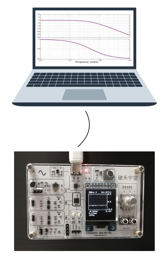
This project utilizes the ADC sampling function of the STM32G031 board to collect voltage signals from analog circuits and sends them to the host computer via UART. The powerful computing capability of the host computer is used to perform FFT on the data, calculating the amplitude and phase frequency characteristics and plotting the curves for display.

2

Design Plan

• Main Control Chip: STM32G031 (Cortex-M0+ core, 64MHz, integrated 12-bit ADC)
• Signal Source: Onboard microphone generator module (for generating audio signals)
• Data Transmission: USB to serial module (CH340 or STM32 built-in USB-CDC)
• Peripheral Functions: TIM1 timer (for precise timing to trigger ADC), ADC channel (to collect microphone analog signals)

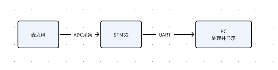
Block diagram and project design ideas introduction

Design Ideas

• Hardware Configuration: Configure TIM1 timer (10kHz interrupt, 0.1ms period), ADC channel (single sampling mode), and serial communication parameters using STM32CubeMX.
• Software Logic: TIM1 interrupt triggers ADC sampling, data is read via DMA or polling, and sent to the PC via serial.
• Host Computer Processing: After receiving the data, the Python script performs FFT analysis based on a 10kHz sampling rate, calculates amplitude and phase response, and dynamically plots the Bode plot through a GUI.

3

Software Introduction

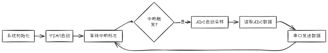
Software Flowchart

Key Code

1. TIM Configuration Function

void MX_TIM1_Init(void){
  /* USER CODE BEGIN TIM1_Init 0 */
  /* USER CODE END TIM1_Init 0 */
  TIM_ClockConfigTypeDef sClockSourceConfig = {0};  TIM_MasterConfigTypeDef sMasterConfig = {0};
  /* USER CODE BEGIN TIM1_Init 1 */
  /* USER CODE END TIM1_Init 1 */  htim1.Instance = TIM1;  htim1.Init.Prescaler = 63999;  htim1.Init.CounterMode = TIM_COUNTERMODE_UP;  htim1.Init.Period = 65535;  htim1.Init.ClockDivision = TIM_CLOCKDIVISION_DIV1;  htim1.Init.RepetitionCounter = 0;  htim1.Init.AutoReloadPreload = TIM_AUTORELOAD_PRELOAD_DISABLE;  if (HAL_TIM_Base_Init(&htim1) != HAL_OK)  {    Error_Handler();  }  sClockSourceConfig.ClockSource = TIM_CLOCKSOURCE_INTERNAL;  if (HAL_TIM_ConfigClockSource(&htim1, &sClockSourceConfig) != HAL_OK)  {    Error_Handler();  }  sMasterConfig.MasterOutputTrigger = TIM_TRGO_RESET;  sMasterConfig.MasterOutputTrigger2 = TIM_TRGO2_RESET;  sMasterConfig.MasterSlaveMode = TIM_MASTERSLAVEMODE_DISABLE;  if (HAL_TIMEx_MasterConfigSynchronization(&htim1, &sMasterConfig) != HAL_OK)  {    Error_Handler();  }
  /* USER CODE BEGIN TIM1_Init 2 */
  /* USER CODE END TIM1_Init 2 */
}

2. PYTHON Code (Partial)

import serial
from collections import deque
import numpy as np
import matplotlib.pyplot as plt
import matplotlib.animation as animation
from threading import Thread, Lock

# Serial Configuration
SERIAL_PORT = 'COM6'
BAUD_RATE = 115200
SAMPLE_RATE = 10000  # Sampling frequency 1kHz
BUFFER_DURATION = 5  # Data buffer duration (seconds)

# Global Variables
raw_buffer = deque(maxlen=int(BUFFER_DURATION * SAMPLE_RATE))  # Raw data buffer
lock = Lock()  # Thread lock

def serial_reader():    # Serial data reading thread
    ser = serial.Serial(SERIAL_PORT, BAUD_RATE, timeout=0.1)
    while True:
        try:
            # Read a line of data
            line = ser.readline()
            if line:  # If data is read
                # Convert binary data to uint32_t
                value = int.from_bytes(line.strip(), byteorder='little', signed=False)
                with lock:
                    raw_buffer.append(value)
        except (ValueError, serial.SerialException):
            pass

def update_plot(frame):
    # Real-time update of Bode plot
    with lock:
        data = np.array(raw_buffer)
    if len(data) < 100:  # At least 100 data points to update
        return
    # FFT Calculation
    N = len(data)
    T = 1.0 / SAMPLE_RATE  # Sampling period
    yf = np.fft.rfft(data - np.mean(data))  # Remove DC component
    xf = np.fft.rfftfreq(N, T)
    # Calculate Amplitude Frequency Characteristics
    magnitude = 20 * np.log10(np.abs(yf) / N * 2)  # Convert to dB
    # Calculate Phase Frequency Characteristics
    phase = np.angle(yf) * 180 / np.pi  # Convert to degrees
    # Plot Bode Diagram
    ax1, ax2 = fig.axes  # Get subplot axes
    ax1.clear()
    ax2.clear()
    ax1.semilogx(xf[1:], magnitude[1:])  # Exclude 0Hz component
    ax1.set_xlabel('Frequency [Hz]')
    ax1.set_ylabel('Magnitude [dB]')
    ax1.set_title('Real-time Bode Diagram')
    ax1.grid(True, which="both", ls="--")
    ax1.set_xlim(1, SAMPLE_RATE//2)  # Display range from 1Hz to Nyquist frequency
    ax2.semilogx(xf[1:], phase[1:])  # Exclude 0Hz component
    ax2.set_xlabel('Frequency [Hz]')
    ax2.set_ylabel('Phase [degrees]')
    ax2.grid(True, which="both", ls="--")
    ax2.set_xlim(1, SAMPLE_RATE//2)  # Display range from 1Hz to Nyquist frequency
if __name__ == '__main__':    # Start serial reading thread
    Thread(target=serial_reader, daemon=True).start()
    # Configure real-time plotting
    fig, (ax1, ax2) = plt.subplots(2, 1, figsize=(10, 12))  # Create subplots
    ani = animation.FuncAnimation(fig, update_plot, interval=10000//SAMPLE_RATE)
    # Show window
    plt.tight_layout()
    plt.show()

4

Challenges Encountered in the Project

Issue 1: TIM1 Interrupt Cycle ErrorPhenomenon: The actual deviation of the 0.1ms interrupt is significant.Solution: Adjust the prescaler and reload value, calibrated using an oscilloscope.Issue 2: Insufficient ADC Sampling TimePhenomenon: Distortion in high-frequency signal sampling.Solution: Reduce ADC clock division and optimize sampling period.Issue 3: Serial Data LossPhenomenon: Data loss during string transmission at high frequencies.Solution: Directly transfer via DMA.

5

Simulation vs Actual Waveform

Simulation link: https://www.eetree.cn/short/28ujfdrc

Without added noise inputWith added noise inputActual MeasurementMeasured amplitude and phase frequency characteristicsAnalyzing the reasons for the differences between simulation results and actual resultsIt may be due to the influence mechanism of environmental noise on high-frequency Bode plots. The signals collected by the microphone are essentially sound pressure signals, which are easily disturbed by environmental noise, especially the differences in high-frequency bands may be related to the following noise factors:

• Noise Types

• Broadband Noise: Such as airflow, electronic device switching noise (fans, power ripple).
• Narrowband Noise: Interference at specific frequencies (such as 50/60Hz power frequency, WiFi/Bluetooth RF interference).
• Mechanical Noise: Microphone vibration or contact noise (such as tapping, friction).

• High-Frequency Sensitivity:High-frequency signals (such as >3kHz) typically have lower sound pressure energy. If environmental noise is superimposed, the signal-to-noise ratio (SNR) sharply decreases, causing noise energy to mask the real signal during FFT analysis, resulting in fluctuations in the amplitude frequency curve or phase confusion.

6

Insights and Reflections

1. Gains

• Mastered the method of quickly configuring peripherals using STM32CubeMX and gained a deep understanding of the collaboration between timers and ADC.
• Practiced data interaction between Python and embedded systems, familiarized with the application of FFT algorithms in frequency domain analysis.

2. Improvement Suggestions

• DMA + double buffering mode can be introduced to improve ADC efficiency.
• The host computer interface can be implemented using PyQt or Tkinter for a more user-friendly interaction.

3. Opinions

• The code generated by STM32CubeMX needs to be combined with manual optimizations (such as interrupt priority) to avoid resource conflicts.

That concludes the introduction to the “Bode Plot of Analog Circuits Based on STM32” project! Feel free to click “Read Original” to download the code and experience the project. The issues and challenges encountered by the author also provide references for everyone, and be sure to pay attention to these points during practice.

If you also want to participate in the activities of Hard Grain, feel free to join the group. The new activity RP2350B is now online, and you can place an order to participate at any time.

NEWS

EETREE

Click Read Original to view this project