Only 3.14% of the world is concerned about
Explode Knowledge
If robots are like seeds, then the show “Robot Arena” is the sower. In the show, different contestants control robots, showcasing various skills on the arena—collisions, rolling, prying, and spitting fire, all of which are dazzling and ignite various fantasies about robots.
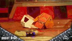
Image from https://giphy.com/gifs/
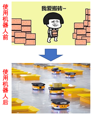
Today, robots are widely used, and robotic technology is continuously penetrating various fields of human activity, such as robotic sorting systems and ubiquitous drones.
For example, robotic sorting systems significantly enhance the efficiency of logistics companies in delivering goods:
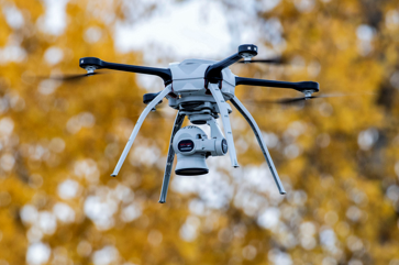
Another example is drones. While sorting robots are still the core secrets of major logistics companies, rarely seen like celestial beings, drones have already become the friendly neighbor, adorning our lives:
The development of robots will not stop here. Since 2020, the concept of new infrastructure has become popular, and its three main directions are closely related to the robotics industry. Educational robots, delivery robots, emotional robots, and autonomous driving technology are all important next steps for robotics and automation technology:
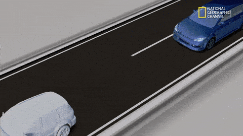
GIF from National Geographic
There is a classic line in the Galaxy Tutoring Class: “My child is attending the best tutoring class in the world, the Galaxy Tutoring Class.” Today, MATLAB brings you the universe’s strongest robot tutoring class, teaching you step by step how to build your own robot!
Many people think of MATLAB as a mathematical or educational software. In fact, MATLAB was initially widely adopted in the field of control engineering, and later developed various leading-edge algorithm packages and toolboxes, which have been widely adopted by universities worldwide as mathematical education software [1]. Are you ready to enter the robot tutoring class?
Step 1: Install the Robotics Toolbox
To do a good job, one must first sharpen their tools. We first need to install MATLAB’s Robotics System Toolbox. We can either download it from the MathWorks official website [2] or open the main MATLAB interface and click on the “Add-Ons” option.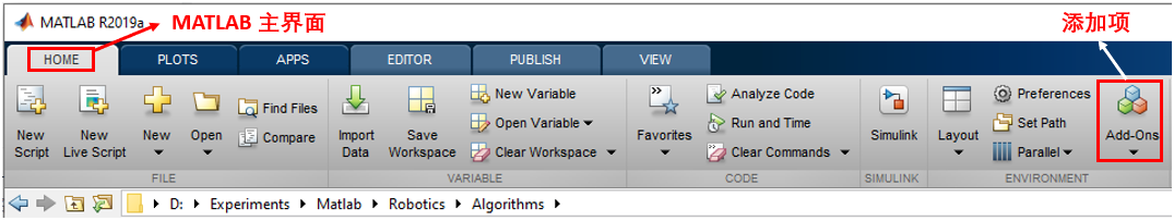 Then, enter “Robotics System Toolbox” in the search bar and install it from the first search result:
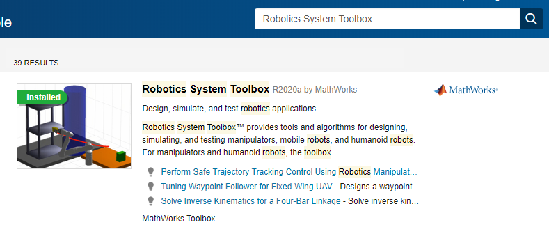 The software has been updated to the latest version R2020a, adding more features. You can try it out. After the installation is complete, open MATLAB and enter
>> ver
If you can find the following information
Robotics System Toolbox Version 2.x (Rxxxxx)
Then congratulations, the Robotics Toolbox has been successfully installed!
Step 2: What kind of robot do you want? Modeling is key
The first robot we want to design is a mechanical arm that can rotate freely. In MATLAB, a mechanical arm is composed of different links (Link) connected by joints (Joint). Depending on their activity state, joints can be classified into rotational and translational, as the names imply [2]: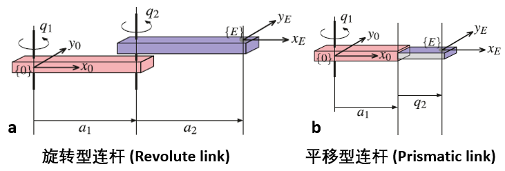 For simplicity, we will first create a three-link mechanical arm:
% Set DH parameters
dhparams = [0     pi/2  0     0;
              0.4318  0       0       0;
            ];
robot = rigidBodyTree; % Initialize the mechanical arm
body1 = rigidBody( 'body1' ); % Define the first link
jnt1 = rigidBodyJoint( 'jnt1' , 'revolute' ); % Define the first joint
setFixedTransform(jnt1,dhparams(1,:), 'dh' );
body1.Joint = jnt1; % Attach the joint to the base
addBody(robot,body1, 'base' ); % Define the mechanical arm as the robot's base

% Add the second and third links
body2 = rigidBody( 'body2' );
jnt2 = rigidBodyJoint( 'jnt2' , 'revolute' );
body3 = rigidBody( 'body3' );
jnt3 = rigidBodyJoint( 'jnt3' , 'revolute' );
setFixedTransform(jnt2,dhparams(2,:), 'dh' );
setFixedTransform(jnt3,dhparams(3,:), 'dh' );
body2.Joint = jnt2;
body3.Joint = jnt3;
The above dhparams is an n*4 matrix (where n is the number of links), known as DH parameters (Denavit–Hartenberg parameters). Each row of dhparams consists of [a alpha d theta] four variables, which represent:
- a: the offset of the joint (in the direction of the vertical link)
- alpha: the joint twist angle (the angle perpendicular to the plane formed by two links)
- d: the extension of the joint (in the direction of the link)
- theta: the initial rotation angle of the joint (the angle parallel to the plane formed by two links)
If you accidentally forget what our robot looks like, the following command
showdetails(robot)
can help us recall its basic features: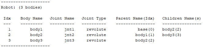 By entering the following command, we can see the true face of the mechanical arm:
addBody(robot,body2, body1 )
addBody(robot,body3, body2 )
show(robot); % Plot
 Since we have only built the most basic links and joints, this mechanical arm is inevitably a bit skinny. However, if we enlarge the above image, we can see the names, numbers, and types of each link and joint:
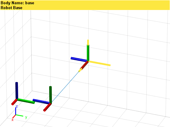 Additionally, we can assign parameters such as mass, moment of inertia, and inertia matrix to the links and joints. Due to space limitations, this will be omitted here. Interested readers can refer to links [1] or [2]. The best way to understand the above concepts is to adjust the parameters in the code one by one and observe the changes in results.
Step 3: Look! It moves slowly with its left and right hands!
We already know how to build a simple robot using MATLAB. However, this robot, built in such a way, is no different from a toy built with building blocks by a child—since it is a robot made with software, we naturally hope it can move. Taking the third-generation robotic arm from the Canadian company Kinova as an example, let’s see how MATLAB can make this arm move.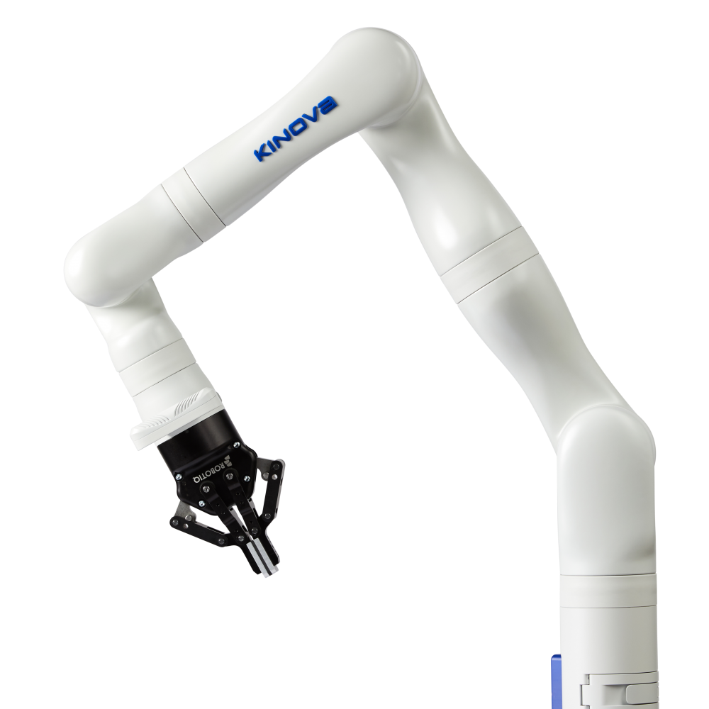 Image from https://www.kinovarobotics.com/en/products/gen3-robotIn the MATLAB interface, enter
>> robot = loadrobot("kinovaGen3");
>> showdetails(robot)
We can see the output as follows 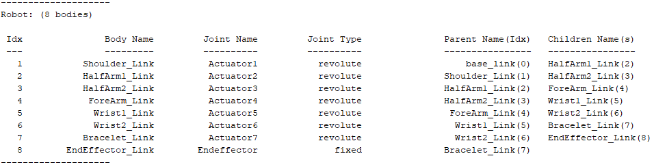 It is not difficult to see that the third-generation Kinova is composed of 8 links and 8 joints. If we want to know the information of a specific link, for example, the link named “Shoulder_Link”, we can sequentially enter
>> robot.getBody( 'Shoulder_Link' ).Joint
>> robot.getBody( 'Shoulder_Link' ).Joint.JointToParentTransform
>> robot.getBody( 'Shoulder_Link' ).Joint.ChildToJointTransform
to query the joint belonging to that link, as well as the transformation matrices from the parent link and to the child link. In this way, we can reconstruct the third-generation Kinova robotic arm!Now we have two methods to make the robotic arm move. The first method is to change the joint rotation angles, known as Forward Kinematics; the second method is to specify the end position of each link, known as Inverse Kinematics. Forward kinematics allows for direct control of the robotic arm, while inverse kinematics is more beneficial for directly specifying tasks for the robotic arm, such as picking up a package at a certain location, etc. Both methods have their advantages.Readers with a geometric background know that rigid body transformations in n-dimensional Euclidean space can be divided into translation, rotation, and reflection, which can be represented by group actions or matrices. The group composed of these three actions is called the Euclidean Group (E(n)), because the elements in E(n) can be represented by matrices, so the subgroup of the n+1 dimensional matrix group E(n) (specific explanation can be seen in the figure below). The subgroup of E(n) composed only of translation and rotation (excluding reflection) is called the special Euclidean group, denoted as SE(n).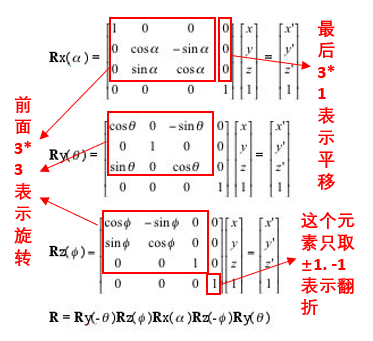 Next, we will use the inverse kinematics function inverseKinematics in MATLAB to make the robotic arm move. We only need to define the positions, velocities, and accelerations of several path points that the robotic arm needs to pass through, and MATLAB can calculate the entire path taken by the robotic arm, as well as the velocity and acceleration at each moment by inverting the special Euclidean group.
% Initial joint rotation angles and initial positions
positions = [2*pi, 0.2619, pi, 4.0142, 2*pi, 0.9598, pi/2];
config = homeConfiguration(robot);
for k = 1:length(positions)
    config(k).JointPosition = positions(k);
end
% Define the path points that the robotic arm needs to pass through, along with corresponding velocity and acceleration information
waypoints = [0.5639 0.0013 0.4336]  + [-0.1 0.2 0.4 ; -0.2 0 0.1 ; -0.1 -0.2 0.4 ;];
waypointTimes = 0:4:8;
ts = 0.2;
trajTimes = 0:ts:waypointTimes(end);
waypointVels = 0.1 *[ 0  1  0; -1  0  0; 0 -1  0;];
waypointAccels = zeros(size(waypointVels));
waypointAccelTimes = diff(waypointTimes)/4;
[q,qd,qdd] = trapveltraj(waypoints,numel(trajTimes), ...
             AccelTime ,repmat(waypointAccelTimes,[3 1]), ...
              EndTime ,repmat(diff(waypointTimes),[3 1]));
% Plot initial state
%% Plot--robotic arm
show(gen3,config, 'Frames' , 'off' , 'PreservePlot' , false);
hold on
%% Plot--path initialization
hTraj = plot3(waypoints(1,1),waypoints(2,1),waypoints(3,1), 'b.-' );
set(hTraj, 'xdata' , q(1,:), 'ydata' , q(2,:), 'zdata' , q(3,:));
%% Plot--path points
plot3(waypoints(1,:),waypoints(2,:),waypoints(3,:), 'ro' , 'LineWidth' ,2);
set(gca, 'Position' , [-.2, -.2, 1.5, 1.5]);
xlim([-1 1]), ylim([-1 1]), zlim([0 1.2]);
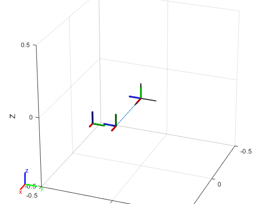
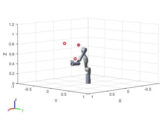 The initial position of the robotic arm. The red dots indicate the path points the robotic arm needs to pass through.
% Initialize the inverse kinematics equation for the robotic arm
ik = inverseKinematics( 'RigidBodyTree' ,robot);
ikWeights = [1 1 1 1 1 1];
ikInitGuess = robot.homeConfiguration; % Randomly set an initial state
% Make the robot move!
for idx = 1:numel(trajTimes)
    % Solve the inverse kinematics equation
    tgtPose = trvec2tform(q(:,idx) );
    [config,info] = ik( 'EndEffector_Link' , tgtPose,ikWeights,ikInitGuess);
    ikInitGuess = config; % Use the previous state as the initial value for the next moment
    % Plot the robot's dynamics
    show(robot,config, 'Frames' , 'off' , 'PreservePlot' , false);
    title([ 'Trajectory at t = ' , num2str(trajTimes(idx))])
    drawnow
end
The final trajectory plot is as follows: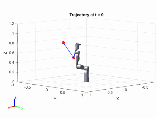 Interested readers can modify the parameters in the above code (such as the positions of the path points, the speed and acceleration of the robotic arm, etc.) to see how the results change.
Advanced Intelligence
In practical use, in addition to making robots move, we also need to give them autonomy. In this section, we hope the robot has the ability for path planning and obstacle avoidance, let’s witness what advanced intelligence is.We take the Simultaneous Localization and Mapping (SLAM) algorithm as an example. This algorithm can be implemented through the famous Kalman Filter. In many engineering applications such as radar, sonar, weather forecasting, rocket launches, computer vision, and control theory, the Kalman filter is indispensable.From an abstract perspective, the Kalman filter is merely a device that continuously adjusts the machine’s state based on external environmental measurements. Let the machine state x (position, velocity, etc.), the external environmental variables measured by the sensor be z (temperature, air pressure, etc.), and the controllable variables be u (emission frequency of electromagnetic waves, direction of movement, etc.), v and w represent the errors of the machine and sensor, respectively, then the Kalman filter can be expressed as a mathematical model: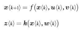 k represents discrete moments. If f and h are linear matrices, then directly taking the partial derivatives of the above two equations with respect to x and z, and then updating the values of x and z will suffice (F_a, H_a represent the partial derivative vectors of f and h with respect to variable a):
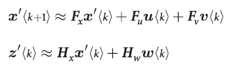 If f and h are not linear, due to the accumulation of error terms, directly linearizing will inevitably lead to greater errors. Therefore, a two-stage algorithm called Predict-Update is used to solve the non-linear Kalman filtering problem—in the prediction phase, we not only need to predict the machine’s state x but also the Kalman filter’s matrix P. This algorithm is called Extended Kalman Filter (EKF), which is the soul of SLAM. Interested readers can refer to literature [2].
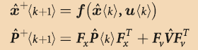 P<k> is the covariance matrix of the Kalman filter at time k, which plays a role in updating variable x.Is the derivation process giving you a headache? Let’s take a look at the code and implementation process!
% Initialize the robot and starting point, endpoint
% Our goal is to ensure the robot can successfully avoid obstacles and reach the endpoint
map = LandmarkMap(20, 10); % 10*10 map, 20 obstacles
V = diag([0.005, 0.5*pi/180].^2); % Error matrix for the robot (for each step)
robot = Bicycle( 'covar' , V); % Initialize the robot
robot.add_driver( RandomPath(10)); % Define the endpoint
% Define the sensor
% angle: sensor scanning angle range
% range: sensor scanning distance
W = diag([0.1, 1*pi/180].^2); % Error matrix for the sensor (for each step)
sensor = RangeBearingSensor(robot, map,  'covar' , W, ...
    'animate' ,  'angle' , [-pi/2 pi/2],  'range' , 5);
% Initialize EKF and run for 150 steps
P0 = diag([0.005, 0.005, 0.001].^2); % Covariance matrix of the Kalman filter at the initial moment
ekf = EKF(robot, V, P0, sensor, W, []);
ekf.run(150);
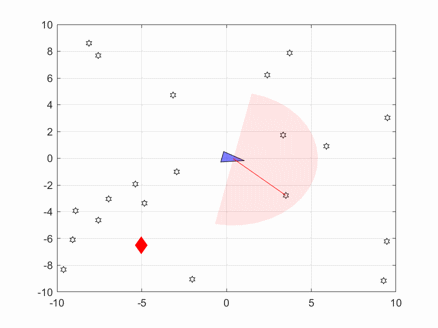 In the above image, the blue triangle represents the robot, the red diamond represents the target, and the pink fan-shaped area represents the sensor scanning range.
Building a Robot? It’s That Simple!
By now, I believe everyone has a sufficient understanding of MATLAB’s Robotics Toolbox. Feeling lonely without a companion?—MATLAB helps you create your own robot! As the robotics industry rapidly develops, it faces various opportunities and challenges. The Robotics Toolbox in MATLAB also needs continuous innovation and research, with improvements needed in the following areas:
- The toolbox does not cover machine vision, so the robot’s sensors can only process non-image environmental information. To give the robot a pair of eyes, you need to download the Computer Vision Toolbox or the Image Processing Toolbox;
- The toolbox cannot utilize big data, which is detrimental to the robot’s growth in today’s highly informationized world. To enable the robot to have big data processing skills, you need the Statistics and Machine Learning Toolbox or the Deep Learning Toolbox.
As a child watching sci-fi movies like “Terminator” and “The Matrix”, I always thought elements like the “Three Laws of Robotics” were far from the real world.However, with the rapid development of computer vision, machine learning, deep learning, and other artificial intelligence-related fields, these elements from sci-fi movies are getting closer to reality. I hope this article can inspire everyone; true learning starts from interest, and one day, you and I will realize our dreams today!

References[1]https://ww2.mathworks.cn/campaigns/products/trials.html?prodcode=RO&s_eid=PEP_23398[2] https://ww2.mathworks.cn/products/robotics.html?s_eid=PEP_23398[3] Cai Zixing, Xie Bin. “Robotics”. Tsinghua University Press; 2000.[4]https://www.mathworks.com/matlabcentral/fileexchange/71130-trajectory-planning-for-robot-manipulators