Word count: 2301, reading time approximately 12 minutes
Hello everyone, this is the Omics Person! In the previous post, we learned how to process the raw FASTQ files generated by sequencers into an analyzable “gene × cell” count matrix. From this article onwards, we will officially enter the exploratory data analysis phase.
Before we start the analysis, we must first choose the right analysis tools. Currently, there are two main analysis ecosystems in the single-cell field: R language’s Bioconductor and Seurat, as well as Python’s scverse. They are all excellent but have different focuses. All subsequent chapters in this series will be based on the scverse ecosystem. This choice is made not only because of its outstanding scalability when handling ultra-large datasets with millions of cells but also because it can seamlessly integrate with Python’s powerful data science and machine learning libraries (such as <span>pandas</span>, <span>scikit-learn</span>, and <span>pytorch</span>). This is crucial for researchers like us who wish to apply cutting-edge models such as deep learning to single-cell data.
In this chapter, we will delve into the three pillars that constitute the <span>scverse</span> ecosystem: <span>AnnData</span>, <span>scanpy</span>, and <span>muon</span>, understanding how they work together to provide a solid foundation for our single-cell exploration journey.
AnnData: The Standard Container for Single-Cell Data
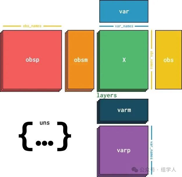
<span>AnnData</span> (Annotated Data) objects are the cornerstone of the <span>scverse</span> ecosystem. We can visualize it as a powerful standard container tailored for single-cell data. Its core design philosophy is to neatly and systematically store all data and metadata generated from a single-cell experiment within the same object, greatly facilitating data management, sharing, and reproducible analysis.
A standard <span>AnnData</span> object (commonly abbreviated as <span>adata</span>) contains the following core data:
- •
<span>adata.X</span>: Core data matrix. This is usually a sparse matrix (<span>cells × genes</span>) that stores the core data we care about most, such as the raw UMI count values. - •
<span>adata.obs</span>: Cell metadata (observations). This is a<span>pandas</span><span>DataFrame</span>, where each row corresponds to a cell and each column is an attribute of the cell, such as its batch, cell cycle stage, quality control metrics (like total UMI count, mitochondrial gene ratio), and final cell type annotations. - •
<span>adata.var</span>: Gene metadata (variables). This is also a<span>DataFrame</span>, where each row corresponds to a gene and each column is an attribute of the gene, such as gene ID, genomic location, and whether it has been filtered as a highly variable gene. - •
<span>adata.obsm</span>: Multi-dimensional representations of cells (multi-dimensional observations). This is a dictionary-like structure used to store the coordinates of cells in different reduced-dimensional spaces, such as PCA, t-SNE, or UMAP results. Each key (like<span>'X_pca'</span>) corresponds to a<span>cells × N</span>-dimensional array. - •
<span>adata.layers</span>: Different versions of the data matrix. This is also a dictionary-like structure that allows us to store multiple different processed versions of the raw data matrix. For example, we can store the raw count values in<span>adata.X</span>, the normalized values in<span>adata.layers['normalized']</span>, and the log-transformed values in<span>adata.layers['log_transformed']</span><code><span>. This layered storage allows us to flexibly call different stages of data during the analysis process without creating multiple </span><code><span>AnnData</span>objects. - •
<span>adata.uns</span>: Unstructured data. This is a dictionary used to store miscellaneous information that does not fit into any of the above categories, such as color schemes for clustering results, parameters for adjacency graphs, or summary information for a specific analysis step.
Scanpy: The Core Tool for Exploratory Analysis
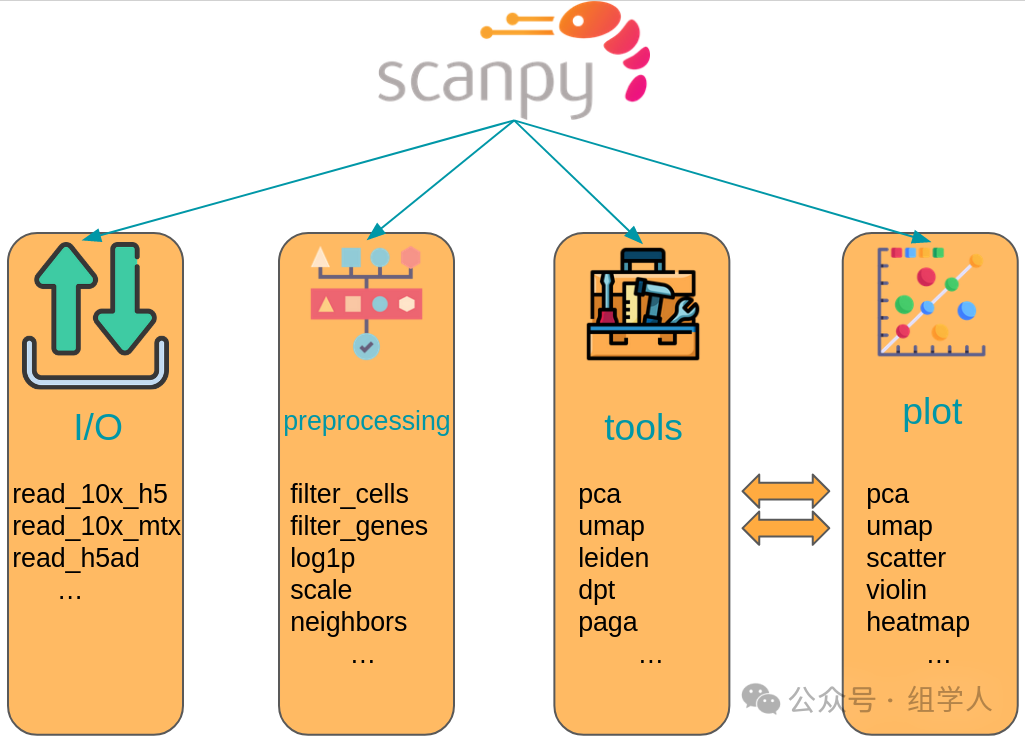
Scanpy provides efficient and user-friendly functions for almost all standard workflows in single-cell analysis, and its API design follows a highly unified and concise philosophy.
<span>scanpy</span>‘s function library can be mainly divided into three core modules, clearly corresponding to the various stages of a typical analysis workflow:
- •
<span>sc.pp.*</span>(preprocessing): Preprocessing module. This includes a series of data preparation steps before formal analysis, such as data filtering, normalization, log transformation, highly variable gene selection, and data scaling. - •
<span>sc.tl.*</span>(tools): Core analysis tools module. This gathers the “hardcore” algorithms of single-cell analysis, such as dimensionality reduction (PCA), constructing neighborhood graphs (Neighbors), clustering (Leiden), calculating UMAP coordinates, and differential gene expression analysis. - •
<span>sc.pl.*</span>(plotting): Visualization module. It provides rich plotting functions that can easily transform data and analysis results from the<span>AnnData</span>object into various beautiful and informative charts, such as UMAP plots, volcano plots, violin plots, etc.
Practical Example: Overview of the Standard Analysis Workflow in Scanpy
Below, using the classic PBMC 3k dataset as an example, we can see how <span>scanpy</span> can complete a standard exploratory analysis workflow with concise and coherent code.
import scanpy as sc

# 1. Load data, scanpy has several classic datasets built-in
adata = sc.datasets.pbmc3k()

# 2. Preprocessing (sc.pp.*)
# 2.1 Basic quality control: filter out low-quality cells and genes
sc.pp.filter_cells(adata, min_genes=200)
sc.pp.filter_genes(adata, min_cells=3)

# 2.2 Normalization and log transformation: bring cells to the same starting line
sc.pp.normalize_total(adata, target_sum=1e4)
sc.pp.log1p(adata)

# 2.3 Select highly variable genes: find the "information-rich" genes that differ the most between cells
sc.pp.highly_variable_genes(adata, min_mean=0.0125, max_mean=3, min_disp=0.5)

# Store the raw data in .raw and slice adata based on highly variable genes, subsequent analysis will only be based on these genes
adata.raw = adata
adata = adata[:, adata.var.highly_variable]

# 2.4 Data scaling: scale the expression of each gene to have a mean of 0 and a variance of 1
sc.pp.scale(adata, max_value=10)

# 3. Core analysis (sc.tl.*)
# 3.1 Dimensionality reduction: calculate principal component analysis (PCA)
sc.tl.pca(adata, svd_solver='arpack')

# 3.2 Construct cell adjacency graph: this is the basis for subsequent clustering and visualization
sc.pp.neighbors(adata, n_neighbors=10, n_pcs=40)

# 3.3 Clustering and visualization coordinate calculation
sc.tl.leiden(adata)  # Leiden clustering
sc.tl.umap(adata)   # UMAP coordinate calculation

# 4. Visualization (sc.pl.*)
# Draw UMAP plot and color based on the expression of key marker genes (B cells, NK cells, T cells)
sc.pl.umap(adata, color=['leiden', 'MS4A1', 'GNLY', 'CD3E'])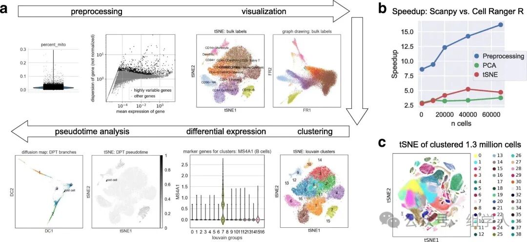
MuData and Muon: Facing the Future of Multi-Modal Analysis
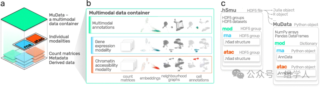
With the advancement of technology, we are increasingly obtaining multiple types of data from the same single-cell experiment, known as multi-modal data (for example, simultaneously measuring a cell’s RNA and surface proteins, i.e., CITE-seq; or simultaneously measuring RNA and chromatin accessibility, i.e., scRNA+scATAC). To address this challenge, the <span>scverse</span> ecosystem elegantly extends its core data structures and tools.
- • MuData: We can think of it as a “container of containers”. It neatly organizes multiple
<span>AnnData</span>objects (one for each modality) from the same cell together.
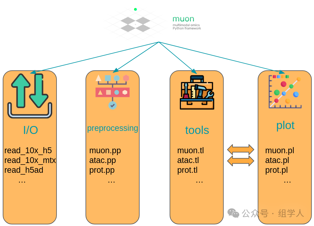
- • muon: The “multi-modal upgraded version” of
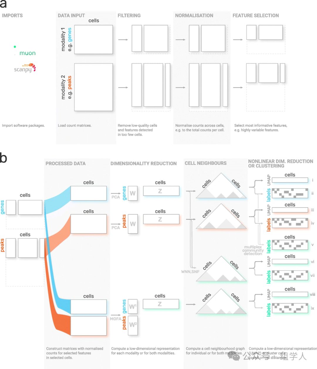
<span>scanpy</span>. It provides an almost identical API to<span>scanpy</span>(<span>mu.pp.*</span>,<span>mu.tl.*</span>,<span>mu.pl.*</span>), but its operation targets are<span>MuData</span>.<span>muon</span>not only allows for independent, modality-specific analysis of each modality in<span>MuData</span>(for example, running PCA on the RNA modality and LSI on the ATAC modality), but it also provides tools for joint analysis of multi-modal data, such as performing weighted nearest neighbor (WNN) analysis to obtain a more comprehensive cell state representation that integrates all modality information.
<span>MuData</span> Object Structure Overview
import muon as mu

# Assume mdata is a pre-loaded CITE-seq MuData object
# mdata
# MuData object with n_obs × n_vars = 7045 × 18076
#   var: 'gene_ids', 'feature_types'
#   2 modalities
#     rna: 7045 x 17938
#       var: 'gene_ids', 'feature_types'
#     prot: 7045 x 138
#       var: 'gene_ids', 'feature_types'

# We can easily access each modality's AnnData object like a dictionary
adata_rna = mdata.mod['rna']
adata_prot = mdata.mod['prot']

# Use muon to perform PCA on the RNA modality
mu.pp.pca(mdata, features_mod='rna')

# Use muon for multi-modal joint neighborhood graph construction and UMAP visualization
mu.pp.neighbors(mdata)
mu.tl.umap(mdata)
mu.pl.umap(mdata, color=['CD3E', 'CD8A', 'CD19']) # Can simultaneously call features from RNA and protein
Summary and Outlook
In this chapter, we learned about the three pillars of the <span>scverse</span> ecosystem:
- • AnnData: A standardized data “container” that ensures orderly and reproducible analysis.
- • Scanpy: A powerful analysis “Swiss Army knife” that provides a complete workflow from preprocessing to visualization.
- • MuData/Muon: A future-oriented multi-modal analysis framework that allows us to understand cells from a more integrated perspective.
With mastery of this core toolkit, we possess a powerful “tool” for exploring the single-cell world. In the upcoming posts, we will utilize the <span>scverse</span> ecosystem to delve into each specific step of single-cell analysis, from quality control and normalization to clustering and annotation, gradually revealing the biological stories behind the data.
References
- • [1] Wolf, F. A., Angerer, P., & Theis, F. J. (2018). SCANPY: large-scale single-cell gene expression data analysis. Genome biology, 19(1), 1-5.
- • [2] Virshup, I., Rybakov, S., & Theis, F. J. (2021). AnnData and MuData: data structures for single-cell and multi-modal genomics. bioRxiv.
- • [3] Hafemeister, C., & Satija, R. (2019). Normalization and variance stabilization of single-cell RNA-seq data using regularized negative binomial regression. Genome biology, 20(1), 1-15.
Thank you for following, liking, sharing, and commenting. Your support is the motivation for my continued creation!