1. Quality Control of Raw Data
The processing of raw data in single-cell sequencing converts the FASTQ files output from sequencers into a more analyzable format, such as a count matrix. This count matrix represents the estimated unique molecular counts for each gene in each quantified cell, sometimes categorized based on the inferred splicing status of each molecule. The count matrix serves as the foundation for various downstream analyses.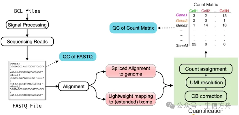
2. Alignment and Mapping
Mapping or alignment is a critical step in single-cell data processing, involving the determination of potential source loci for each sequencing fragment, such as genomic or transcriptomic locations that closely match the read sequences. In single-cell sequencing protocols, the raw sequence files typically include: Cell Barcodes, Unique Molecular Identifiers, and Raw cDNA sequences. scRNA-seq datasets often involve hundreds of millions to billions of reads, making this step computationally challenging. Many existing RNA-seq aligners are unpredictable and cannot inherently interpret features unique to scRNA-seq, such as cell barcodes, UMIs, or their positions and lengths. To address the challenges of aligning and mapping scRNA-seq data, several specialized tools have been developed: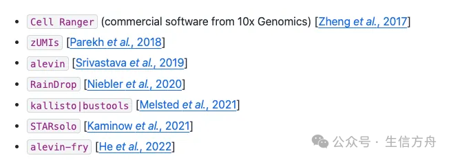 These tools are specifically designed to handle single-cell RNA sequencing (scRNA-seq) data, with capabilities for aligning reads, parsing technical sequences (such as cell barcodes and UMIs), demultiplexing, and UMI resolution. While they often provide simplified user interfaces, the internal implementation methods vary significantly: some tools generate traditional intermediate files, such as BAM files, which require further processing, while others operate entirely in memory or use compact intermediate representations to minimize input/output operations and reduce computational overhead. Overall, these tools differ in their specific algorithms, data structures, and trade-offs in time and space complexity, but their approaches can generally be categorized along two dimensions: the type of mapping performed and the type of reference sequence used.
3. Types of Mapping
The main mapping algorithms used for sc/snRNA-seq data include splice-aware alignment, continuous alignment, and lightweight mapping. Alignment-based methods utilize various heuristic strategies to identify potential source loci for reads, followed by scoring nucleotide-level alignments between reads and reference sequences using dynamic programming algorithms to determine the best match. Global alignment compares the entire query sequence with the reference sequence, while local alignment focuses on aligning subsequences. Short read alignments typically employ semi-global alignment methods, also known as “fitting” alignments, which align most of the query sequence with a substring of the reference sequence. Additionally, “extension” alignments can achieve “soft-clipping” to reduce penalties for mismatches, insertions, or deletions occurring at the start or end of reads. Although these variants alter the rules for dynamic programming recursion and backtracking, they do not fundamentally change the overall complexity. Lightweight mapping methods can significantly improve speed; however, they do not provide easily interpretable score-based assessments to determine match quality, making it more challenging to evaluate alignment confidence.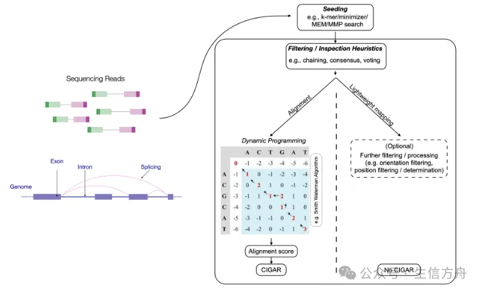
4. Mapping Based on Different Reference Sequences
There are three main types of reference sequences: 1. Whole genome (usually annotated); 2. Annotated transcriptome; 3. Enhanced transcriptome.
Mapping to the Complete Genome
The first type of reference sequence used for alignment is the entire genome of the target organism, typically considering annotated transcripts during the alignment process. Tools like zUMIs, Cell Ranger, and STARsolo adopt this approach. Since many reads originate from spliced transcripts, this method requires alignment algorithms capable of “recognizing splicing” to split alignments at one or more splice sites. A key advantage of this method is its ability to handle reads originating from any position in the genome, not just annotated transcripts. Additionally, because a whole genome index is constructed, reporting reads aligned to known spliced transcripts incurs almost no additional overhead when outputting reads overlapping with introns or falling in non-coding regions, making this method equally effective in single-cell and single-nucleus data analyses. Another benefit is that reads aligned to regions outside annotated transcripts, exons, or introns can also be recorded, supporting the supplementation and extension of quantified loci in subsequent analyses.
Mapping to the Spliced Transcriptome
To reduce the computational resource consumption associated with aligning reads to the entire genome, a widely adopted alternative method is to use only the sequences of annotated transcripts as references. Since most single-cell experiments are conducted in model organisms like mice or humans, which have relatively well-annotated transcriptomes, transcriptome-based quantification methods can achieve coverage comparable to genome-based methods. Compared to the genome, transcript sequences are much smaller, significantly reducing the computational resources required for alignment. Furthermore, since splicing patterns are already reflected in the transcript sequences, this method does not require complex splicing alignments, only needing to find continuous alignments or mappings in the reads. In other words, reads can be mapped through continuous alignments, making both alignment-based and lightweight mapping methods applicable in transcriptome-based scenarios.
Although these methods significantly reduce the memory and time required for alignment and mapping, they cannot capture reads originating from outside the spliced transcriptome, making them unsuitable for processing single-nucleus data. Even in single-cell experiments, reads from regions outside the spliced transcriptome can constitute a considerable proportion, and increasing evidence suggests that these reads should be included in subsequent analyses. Additionally, when combined with lightweight mapping methods, the short sequences shared between the spliced transcriptome and the actual regions of the genome producing reads may lead to erroneous mappings, resulting in misleading or even biologically unreasonable gene expression estimates.
Mapping to the Enhanced Transcriptome
To account for reads originating from outside spliced transcripts, additional reference sequences can be added to the spliced transcript sequences, such as full-length unspliced transcripts or spliced-out intron sequences. Compared to aligning to the whole genome, this method can achieve better, faster, and more memory-efficient alignments while still capturing many reads that would otherwise be missed. It allows for better allocation of more reads compared to using only the spliced transcriptome, and when combined with lightweight mapping methods, it can significantly reduce erroneous mappings. Enhanced transcriptomes are widely used in methods that do not perform whole genome alignments, especially suitable for single-nucleus data processing and RNA velocity analysis (see RNA velocity). These enhanced reference sequences can be constructed for all commonly used methods that do not rely on whole genome spliced alignments.
5. Correction of Cell Barcodes
Droplet-based single-cell separation systems, such as those provided by 10x Genomics, have become important tools for studying the causes and effects of cellular heterogeneity. In these separation systems, the RNA of each captured cell is extracted in aqueous droplets, simultaneously encapsulated with barcoded microbeads. These microbeads use unique oligonucleotides—referred to as cell barcodes (CBs)—to label the RNA content of individual cells, which are then sequenced along with cDNA fragments obtained from the reverse transcription of RNA. The microbeads contain a high diversity of DNA barcodes, allowing for the parallel barcode labeling of the molecular content of cells and demultiplexing the sequencing reads on a computer into individual cell groups.
Types of Errors in Barcodes
Key types of errors include: 1. Doublets/Multiplets: A single barcode may correspond to multiple cells, leading to an underestimation of cell numbers. 2. Empty droplets: Some droplets may not contain encapsulated cells, but RNA from the environment may be labeled and sequenced by the barcode, leading to an overestimation of cell numbers. 3. Sequence errors: Errors introduced during PCR amplification or sequencing may distort barcode counts, potentially leading to both underestimation and overestimation. To address these issues, computational tools for demultiplexing RNA-seq reads into specific cell groups utilize various diagnostic metrics to filter out artifacts or low-quality data. Numerous methods are already available to remove environmental RNA contamination, detect doublets/multiplets, and correct cell barcode errors based on nucleotide sequence similarity. To address these issues, computational tools for splitting RNA-seq reads into specific cell bins utilize various diagnostic metrics to filter out artifacts or low-quality data. A large number of methods are available to remove environmental RNA contamination, detect doublets, and correct cell barcode errors based on nucleotide sequence similarity.
6. UMI Resolution
After the correction of cell barcodes (CBs), sequencing reads are either discarded or assigned to a corrected CB. Researchers aim to quantitatively analyze the abundance of each gene within each corrected CB. Due to the amplification bias issues discussed in transcript quantification, reads must be deduplicated based on their UMI to assess the actual number of molecules sampled. Additionally, several other complex factors pose challenges to this estimation. The goal of the UMI deduplication step is to identify the set of reads and UMIs captured and sequenced from each original (pre-PCR) molecule in each cell during the experiment. The result of this process is to assign a molecular count for each gene in each cell, which is then used as an estimate of the original expression level of that gene for downstream analyses. Researchers refer to this process as UMI resolution, which infers the actual observed number of molecules in each gene by examining the observed UMI set and its associated aligned reads.
Necessity of UMI Resolution
UMI errors: These errors occur when errors are introduced during the sequencing of the UMI tags read. Common UMI errors include nucleotide substitutions during the PCR process and read errors during sequencing. Multi-mapping: This issue arises when a read or UMI belongs to multiple reference genomes (e.g., multi-gene reads/UMIs). This problem leads to ambiguity regarding the gene source of multi-gene reads/UMIs, resulting in uncertainty in the pre-PCR molecular count samples for those genes. Simply discarding multi-gene reads/UMIs may lead to data loss or introduce bias among genes that tend to produce multi-mapping reads, such as sequence-similar gene families. There are also challenges not discussed here, such as “convergent” and “divergent” UMI conflicts. The following situation is considered a convergent conflict: the same UMI is used to label two different pre-PCR molecules from the same gene in the same cell. When two or more different UMIs from the same pre-PCR molecule occur (e.g., due to sampling from multiple primer binding sites on that molecule), it is considered a divergent conflict. Expected convergent UMI conflicts are rare, so their impact is usually minimal. Additionally, transcript-level alignment information can sometimes be used to resolve such conflicts. Divergent UMI conflicts primarily occur in intronic regions of unspliced transcripts, and how to address the issues they pose remains an active area of research.
7. Quality Control of the Matrix
Once the count matrix is generated, quality control (QC) assessments are necessary. Quality control typically includes several different assessment stages. The most basic are some global metrics to help judge the overall quality of the sequencing itself. These metrics include: the total proportion of reads aligned to the reference sequence, the distribution of different UMIs detected per cell, the distribution of UMI deduplication rates, and the distribution of the number of genes detected per cell, among others. Similar metrics are usually recorded and output by the quantification tools themselves, as these values can naturally be calculated during the processes of read alignment, cell barcode correction, and UMI resolution. Likewise, there are tools available to help organize and visualize these basic metrics, such as Loupe Browser, alevinQC, or kb_python reports, depending on the quantification analysis workflow used. In addition to these basic global metrics, the main goal of QC metrics at this stage of analysis is to help determine which cells (CBs) have been sequenced “successfully” and which cells exhibit artifacts that need to be filtered or corrected. Among the more important detections are: empty droplet detection and doublet detection.
8. Representation of Count Data
When the initial processing and quality control of the raw data are completed and subsequent analyses are entered, it is essential to clarify and remember that the cell × gene count matrix is at best an approximate representation of the sequenced molecules in the original sample. Heuristic methods and simplifications are employed at multiple stages of the raw data processing workflow to generate this count matrix. For example, read alignment is not perfect, and cell barcode correction also has errors. The accurate resolution of UMIs is particularly challenging, and UMI issues related to multi-mapping reads are often overlooked. Furthermore, the presence of multiple primer binding sites in unspliced molecules may violate the common assumption of “one molecule corresponds to one UMI.”
9. Using AnnData to Store Single-Modal Data
As previously discussed, after alignment and gene annotation, genomic data is typically summarized into a feature matrix. This matrix has the shape of observations × variables—where in scRNA-seq, observations correspond to cell barcodes, and variables correspond to annotated genes. During the analysis process, the observations and variables of this matrix will be supplemented with computed metrics (e.g., quality control metrics or latent space embeddings) and prior knowledge (e.g., donor source or alternative gene identifiers). In the scverse ecosystem, AnnData is used to associate the data matrix with these annotations. To achieve fast and memory-efficient conversions, AnnData also supports sparse matrices and partial reads. In its core structure, the AnnData object stores a sparse or dense matrix (in the case of scRNA-seq, the count matrix) in X. The dimensions of this matrix are obs_names × var_names, where obs (observations) correspond to cell barcodes, and var (variables) correspond to gene identifiers.
Surrounding this matrix X, AnnData saves annotation information for cells and genes in the obs and var of Pandas DataFrames, respectively. Additionally, AnnData stores the complete computed matrices corresponding to observations or variables in obsm or varm, with dimensions matching them. Graph structures describing relationships between cells and between genes are typically stored in obsp and varp. Any unstructured data that does not fit in the above locations is stored in uns as unstructured data.
Furthermore, multiple versions of X can be stored in layers. A common use case is to save the original, unnormalized count data in the counts layer, while saving the normalized data in the default unnamed layer.
In its core structure, the AnnData object stores a sparse or dense matrix (in the case of scRNA-seq, the count matrix) in X. The dimensions of this matrix are obs_names × var_names, where obs (observations) correspond to cell barcodes, and var (variables) correspond to gene identifiers.
This matrix X is surrounded by the obs and var of Pandas DataFrames, which are used to store annotation information for cells and genes, respectively. Additionally, AnnData stores the complete computed matrices corresponding to observations or variables in obsm or varm, with dimensions matching them. Graph structures describing relationships between cells and between genes are typically stored in obsp and varp. Any unstructured data that does not fit in the above locations is stored in uns as unstructured data.
Moreover, multiple versions of X can be stored in layers. A typical application scenario is to save the original, unnormalized count data in the counts layer, while saving the normalized data in the default unnamed layer.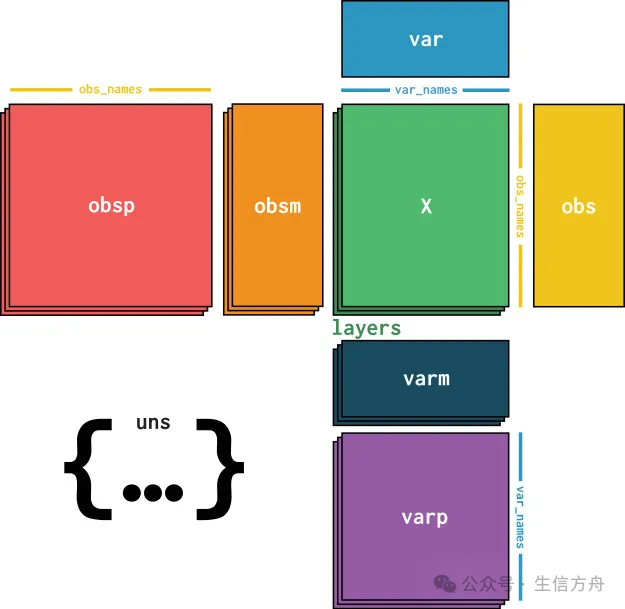
References:
- single-cell-best-practices-zh github: https://github.com/master-XS/single-cell-best-practices-zh/tree/development/jupyter-book/introduction
Note: If you have any questions about the content or find any clear errors, please contact the backend. For more related content, please follow the public account:Bioinformatics Ark.
Conclusion
Welcome to join the “Bioinformatics & Clinical” group chat. If you are interested in joining, please add WeChat:couqiliugeziba321, and please indicate “Organization or School – Major or Direction – Name or Nickname“. We hope that you gain knowledge and joy while joining the group! 🤗
– END –