Three Applications of LoRA in Stable Diffusion: Principles and Code Examples

If you have been following the Stable Diffusion (SD) community, you must be familiar with the term “LoRA”. The SD LoRA models shared by community users can modify the style of SD to produce images in styles such as anime, ink wash, or pixel art. However, LoRA can do more than just change the style of SD; it has other clever uses as well. In this article, we will first briefly learn about the principles of LoRA, then explore three common applications of LoRA in research: 1) restoring a single image; 2) style adjustment; 3) training objective adjustment, and finally read two code implementation examples of SD LoRA based on Diffusers.

Principles of LoRA

Before understanding LoRA, let’s review some concepts related to transfer learning. Transfer learning refers to reusing the knowledge of a previously trained model in a new training session. If you have ever trained a deep learning model yourself, you have probably used transfer learning without realizing it: for example, if you trained a model for 500 steps and found that the results were not ideal, you might have reloaded the model’s parameters and continued training for another 100 steps. The previously trained model is called a pre-trained model, and the process of continuing to train a pre-trained model is called fine-tuning.

Now that we know the concept of fine-tuning, we can understand LoRA. LoRA stands for Low-Rank Adaptation, which is a Parameter-Efficient Fine-Tuning (PEFT) method that only trains a portion of the parameters in the original model during fine-tuning, accelerating the process. Compared to other PEFT methods, LoRA stands out for several obvious advantages:

• From a performance perspective, using LoRA requires storing only a small number of fine-tuned parameters, rather than saving the entire new model. Additionally, the new parameters of LoRA can be merged with the parameters of the original model without increasing the computation time of the model.
• From a functionality perspective, LoRA maintains the “change amount” of the model during fine-tuning. By multiplying the change amount by a mixing ratio between 0 and 1, we can control the degree of modification to the model. Furthermore, multiple LoRA models trained independently based on the same original model can be used simultaneously.

These advantages are reflected in SD LoRA as follows:

• SD LoRA models are generally very small, typically only a few tens of MB.
• The parameters of SD LoRA models can be merged into the SD base model to obtain a new SD model.
• A ratio between 0 and 1 can be used to control the degree of the new style produced by SD LoRA.
• Different styles of SD LoRA models can be mixed in different proportions.

Why does LoRA have these advantages? What does the “low-rank” in LoRA mean? Let’s start with the advantages of LoRA and gradually reveal its principles.

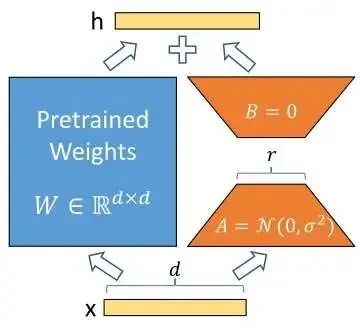
As mentioned earlier, the flexibility of LoRA comes from its maintenance of the change amount of the model during fine-tuning. Therefore, suppose we are modifying a parameter in the model; we should maintain its change amount, represented by the parameter during training. Thus, to control the degree of modification to the model during inference, we simply add a parameter, making the parameter used equal to .

However, doing this still requires recording a parameter matrix that is the same size as the original parameter matrix, which does not qualify as parameter-efficient fine-tuning. To address this, the authors of LoRA proposed the assumption that the information contained in the change amount of the model parameters during fine-tuning is not so large. To represent the change amount with less information, we can decompose into the product of two low-rank matrices:

where is a much smaller number than . Thus, by using two much smaller parameter matrices to maintain the change amount, we not only improve the efficiency of fine-tuning but also maintain the flexibility of describing the fine-tuning process using the change amount. This is the entire principle of LoRA, which is very simple and can be represented by this line of formula.

Having understood the principles of LoRA, let’s revisit the four advantages of LoRA mentioned earlier. The LoRA model is represented by many low-parameter matrices, which can be stored separately and occupy little space. Since it actually maintains the change amount of the parameters, we can either combine it with the parameters of the pre-trained model to obtain a new model to improve inference speed or flexibly combine the new and old models online with a mixing ratio. The last advantage of LoRA is that various LoRA models independently trained based on the same original model can be mixed and used. LoRA can even act on original models modified by other methods, such as SD LoRA supporting SD with ControlNet. This point actually comes from the practical experience of community users. One possible explanation is that LoRA uses low-rank matrices to represent the change amount, and this low-rank change amount happens to be “offset” from the change amounts of other methods, allowing LoRA to modify the model in a direction that does not interfere with other methods.

Finally, let’s learn about the implementation details of LoRA. LoRA has two hyperparameters: in addition to the parameter mentioned above, there is also a parameter called . When implementing the LoRA module, the authors multiplied the modification amount by a coefficient of , that is, for input , the output after adding the LoRA module is . The authors explain that adjusting this parameter is almost equivalent to adjusting the learning rate, and initially setting is sufficient. When we need to repeatedly adjust the hyperparameter , we only need to keep unchanged, and there is no need to modify other hyperparameters (because if is not added, changing will require corresponding adjustments to learning rates and other parameters to maintain the same training conditions). Of course, in practical applications, the hyperparameters of LoRA are easy to adjust. Generally, it is sufficient to set . Since we do not change too much, always setting is enough.

To use LoRA, in addition to determining the hyperparameters, we also need to specify which parameter matrices need to be fine-tuned. When using LoRA in SD, everyone generally fine-tunes all parameter matrices of all multi-head attention modules in the U-Net of SD. That is, fine-tuning the four matrices of the multi-head attention module.

Three Applications of LoRA in SD

LoRA has a wide range of applications in SD research. According to the motivation for using LoRA, we can divide its applications into: 1) restoring a single image; 2) style adjustment; 3) training objective adjustment. By learning these applications, we can better understand the essence of LoRA.

Restoring a Single Image

SD is merely a model for generating arbitrary images. To use SD to edit a given image, we generally need to let SD first learn to generate an identical image and then modify it based on that. However, due to the differences between the training set and the input image, SD may not be able to generate an identical image. The solution to this problem is simple and straightforward: we only use this one image to fine-tune SD, causing SD to overfit on this image. Thus, the output of SD will be very similar to this image.

The earlier work introducing this method to improve the fidelity of the input image is Imagic, which adopted a complete fine-tuning strategy. The subsequent DragDiffusion used the same approach and replaced complete fine-tuning with LoRA. Recently, DiffMorpher, in order to achieve interpolation between two images, not only trained LoRA for the two images separately but also smoothed the image interpolation process through interpolation between the two LoRA.

Style Adjustment

The most popular application of LoRA in the SD community is style adjustment. We hope that SD only generates images in a certain style or of a certain character. For this, we only need to directly train SD LoRA on a training set that meets our requirements.

Since this method of adjusting the style of SD is very direct, there are no specific papers introducing this method. It is worth mentioning that the video model AnimateDiff based on SD uses LoRA to control the perspective transformation of output videos rather than controlling the style.

Since SD stylization LoRA has been widely used, whether it is compatible with SD stylization LoRA determines whether a work is easy to spread in the community.

Training Objective Adjustment

The last application is somewhat returning to the basics. The original application of LoRA was to adapt a pre-trained model to another task. For example, GPT was initially trained on a large corpus and then fine-tuned on a question-answering task. For SD, we can also modify the training objectives of U-Net to enhance the capabilities of SD.

Many related works have used LoRA to improve SD. For example, Smooth Diffusion adds a constraint term to the training objective and performs LoRA fine-tuning to make the latent space of SD smoother. Recently popular fast image generation methods LCM-LoRA also use LoRA to implement a model distillation process that originally acted on all parameters of SD.

Summary of SD LoRA Applications

Although the design starting points of the above three SD LoRA applications are different, they essentially utilize the transfer learning technique of fine-tuning to adjust the data distribution or training objectives of the model. LoRA is just one of many efficient fine-tuning methods; as long as it is a function that fine-tuning can achieve, LoRA can basically achieve it, but LoRA is more lightweight. If you want to fine-tune SD but are worried about insufficient computing resources, using LoRA is definitely the right choice. Conversely, if you want to design a new application using LoRA on SD, you need to think about what fine-tuning SD can achieve.

Diffusers SD LoRA Code Practice

Having looked at the principles, let’s try training LoRA using Diffusers. We will first learn the script for training LoRA with Diffusers, then look at two simple LoRA examples: SD image interpolation and SD image style transfer.

Project URL: https://github.com/SingleZombie/DiffusersExample/tree/main/LoRA

Diffusers Script

We will refer to the SD LoRA documentation in Diffusers https://huggingface.co/docs/diffusers/training/lora, using the official script examples/text_to_image/train_text_to_image_lora.py to train LoRA. To use this script, it is recommended to clone the official repository directly and install the dependencies in the root directory and the text_to_image directory. The version of Diffusers used in this article is 0.26.0; older versions of Diffusers may differ from what is shown in this article. Currently, the official documentation also describes an older version of the code.

git clone https://github.com/huggingface/diffusers
cd diffusers
pip install .
cd examples/text_to_image
pip install -r requirements.txt

This code uses the accelerate library to manage PyTorch training. With the same code, simply modifying the accelerate configuration can achieve single-card or multi-card training. By default, running the Python script with the accelerate launch command will use all GPUs. If you need to modify the training configuration, please refer to the relevant documentation to use the accelerate config command to configure the environment.

Once prepared, let’s start reading the code in examples/text_to_image/train_text_to_image_lora.py. This code is written very understandably, with comments explaining complex parts. We will skip the command-line argument section and start reading from the main function.

Initially, the function configures the accelerate library and the logger.

args = parse_args()
logging_dir = Path(args.output_dir, args.logging_dir)

accelerator_project_config = ProjectConfiguration(project_dir=args.output_dir, logging_dir=logging_dir)

accelerator = Accelerator(
    gradient_accumulation_steps=args.gradient_accumulation_steps,
    mixed_precision=args.mixed_precision,
    log_with=args.report_to,
    project_config=accelerator_project_config,
)
if args.report_to == "wandb":
    if not is_wandb_available():
        raise ImportError("Make sure to install wandb if you want to use it for logging during training.")
    import wandb

# Make one log on every process with the configuration for debugging.
logging.basicConfig(
    format="%(asctime)s - %(levelname)s - %(name)s - %(message)s",
    datefmt="%m/%d/%Y %H:%M:%S",
    level=logging.INFO,
)
logger.info(accelerator.state, main_process_only=False)
if accelerator.is_local_main_process:
    datasets.utils.logging.set_verbosity_warning()
    transformers.utils.logging.set_verbosity_warning()
    diffusers.utils.logging.set_verbosity_info()
else:
    datasets.utils.logging.set_verbosity_error()
    transformers.utils.logging.set_verbosity_error()
    diffusers.utils.logging.set_verbosity_error()

The subsequent code determines whether to manually set the random seed. It is best to keep the default.

# If passed along, set the training seed now.
if args.seed is not None:
    set_seed(args.seed)

Next, the function creates an output folder. If we want to push the model to an online repository, the function will also create a repository. Our project does not need to be uploaded, so we can ignore all args.push_to_hub options. Additionally, if accelerator.is_main_process: indicates that this code block will only be executed by the main process during multi-card training.

# Handle the repository creation
if accelerator.is_main_process:
    if args.output_dir is not None:
        os.makedirs(args.output_dir, exist_ok=True)

    if args.push_to_hub:
        repo_id = create_repo(
            repo_id=args.hub_model_id or Path(args.output_dir).name, exist_ok=True, token=args.hub_token
        ).repo_id

After preparing the auxiliary tools, the function officially begins the training process. Before training, the function will instantiate all processing classes needed, including DDPMScheduler for maintaining intermediate variables in the diffusion model, CLIPTokenizer, CLIPTextModel for encoding input text, AutoencoderKL for compressing images, and UNet2DConditionModel for predicting noise. The parameter args.pretrained_model_name_or_path is the address of Diffusers’ online repository (such as runwayml/stable-diffusion-v1-5) or the local folder of Diffusers models.

# Load scheduler, tokenizer and models.
noise_scheduler = DDPMScheduler.from_pretrained(args.pretrained_model_name_or_path, subfolder="scheduler")
tokenizer = CLIPTokenizer.from_pretrained(
    args.pretrained_model_name_or_path, subfolder="tokenizer", revision=args.revision
)
text_encoder = CLIPTextModel.from_pretrained(
    args.pretrained_model_name_or_path, subfolder="text_encoder", revision=args.revision
)
vae = AutoencoderKL.from_pretrained(
    args.pretrained_model_name_or_path, subfolder="vae", revision=args.revision, variant=args.variant
)
unet = UNet2DConditionModel.from_pretrained(
    args.pretrained_model_name_or_path, subfolder="unet", revision=args.revision, variant=args.variant
)

The function will also set whether the parameter models need to compute gradients. Since we are going to optimize the newly added LoRA model, all pre-trained models do not need to compute gradients. Additionally, the function will automatically set the precision of these models according to the accelerate configuration.

# freeze parameters of models to save more memory
unet.requires_grad_(False)
vae.requires_grad_(False)
text_encoder.requires_grad_(False)

# Freeze the unet parameters before adding adapters
for param in unet.parameters():
    param.requires_grad_(False)

# For mixed precision training we cast all non-trainable weigths (vae, non-lora text_encoder and non-lora unet) to half-precision
# as these weights are only used for inference, keeping weights in full precision is not required.
weight_dtype = torch.float32
if accelerator.mixed_precision == "fp16":
    weight_dtype = torch.float16
elif accelerator.mixed_precision == "bf16":
    weight_dtype = torch.bfloat16

# Move unet, vae and text_encoder to device and cast to weight_dtype
unet.to(accelerator.device, dtype=weight_dtype)
vae.to(accelerator.device, dtype=weight_dtype)
text_encoder.to(accelerator.device, dtype=weight_dtype)

Once the pre-trained models are configured, the function will configure the LoRA module and add it to the U-Net model. Recently, Diffusers updated the way to add LoRA. Diffusers uses Attention processors to describe the computation of Attention. To add LoRA to the Attention module, early versions of Diffusers directly added trainable parameters in the Attention processor. Now, to unify with other Hugging Face libraries, Diffusers uses the PEFT library to manage LoRA. We do not need to focus on the implementation details of LoRA; we only need to write a LoraConfig.

For the LoRA documentation in PEFT, refer to https://huggingface.co/docs/peft/conceptual_guides/lora

LoraConfig has four main parameters: r, lora_alpha, init_lora_weights, target_modules. The meanings of r and lora_alpha have been seen in the previous text; the former determines the size of the LoRA matrix, while the latter determines the training speed. In the default configuration, they are both equal to the same value args.rank. init_lora_weights indicates how to initialize the training parameters, with gaussian being the method used in the paper. target_modules indicates which layers of the Attention module need to add LoRA. Typically, all layers, i.e., the three input transformation matrices to_k, to_q, to_v and one output transformation matrix to_out.0, will have LoRA added.

After creating the configuration, we can create the LoRA module with unet.add_adapter(unet_lora_config).

unet_lora_config = LoraConfig(
    r=args.rank,
    lora_alpha=args.rank,
    init_lora_weights="gaussian",
    target_modules=["to_k", "to_q", "to_v", "to_out.0"],
)

unet.add_adapter(unet_lora_config)
if args.mixed_precision == "fp16":
    for param in unet.parameters():
        # only upcast trainable parameters (LoRA) into fp32
        if param.requires_grad:
            param.data = param.to(torch.float32)

After updating the U-Net structure, the function will try to enable xformers to improve the efficiency of Attention. PyTorch 2.0 also introduced similar Attention optimization techniques. If your GPU performance is limited and your PyTorch version is below 2.0, you might consider using xformers.

if args.enable_xformers_memory_efficient_attention:
  if is_xformers_available():
      import xformers

      xformers_version = version.parse(xformers.__version__)
      if xformers_version == version.parse("0.0.16"):
          logger.warn(
              ...
          )
      unet.enable_xformers_memory_efficient_attention()
  else:
      raise ValueError("xformers is not available. Make sure it is installed correctly")

After processing the U-Net, the function will filter out the model parameters to be optimized, which will be passed to the optimizer later. The filtering principle is simple; if the parameter requires gradients, it is a parameter to be optimized.

lora_layers = filter(lambda p: p.requires_grad, unet.parameters())

Next comes the configuration of the optimizer. The function first configures some minor training options, which can generally be ignored.

if args.gradient_checkpointing:
    unet.enable_gradient_checkpointing()

# Enable TF32 for faster training on Ampere GPUs,
# cf https://pytorch.org/docs/stable/notes/cuda.html#tensorfloat-32-tf32-on-ampere-devices
if args.allow_tf32:
    torch.backends.cuda.matmul.allow_tf32 = True

Then, the selection of the optimizer. We can ignore other logic and directly use AdamW.

# Initialize the optimizer
if args.use_8bit_adam:
    try:
        import bitsandbytes as bnb
    except ImportError:
        raise ImportError(
            "..."
        )

    optimizer_cls = bnb.optim.AdamW8bit
else:
    optimizer_cls = torch.optim.AdamW

Once the optimizer class is selected, the optimizer can be instantiated. The first parameter of the optimizer is the LoRA parameters prepared for optimization, and other parameters are parameters of the Adam optimizer itself.

optimizer = optimizer_cls(
    lora_layers,
    lr=args.learning_rate,
    betas=(args.adam_beta1, args.adam_beta2),
    weight_decay=args.adam_weight_decay,
    eps=args.adam_epsilon,
)

With the optimizer prepared, the next step is to prepare the training set. This script uses Hugging Face’s datasets library to manage datasets. We can read online datasets or read local image folder datasets. In the example project of this article, we will use an image folder dataset. Later, we will learn how to build such a dataset folder. For related documentation, refer to https://huggingface.co/docs/datasets/v2.4.0/en/image_load#imagefolder.

if args.dataset_name is not None:
    # Downloading and loading a dataset from the hub.
    dataset = load_dataset(
        args.dataset_name,
        args.dataset_config_name,
        cache_dir=args.cache_dir,
        data_dir=args.train_data_dir,
    )
else:
    data_files = {}
    if args.train_data_dir is not None:
        data_files["train"] = os.path.join(args.train_data_dir, "**")
    dataset = load_dataset(
        "imagefolder",
        data_files=data_files,
        cache_dir=args.cache_dir,
    )
    # See more about loading custom images at
    # https://huggingface.co/docs/datasets/v2.4.0/en/image_load#imagefolder

When training SD, each data sample needs to contain two pieces of information: image data and corresponding text descriptions. In the dataset dataset, each data sample contains multiple attributes. The following code is used to extract the image and text descriptions from these attributes. By default, the first attribute will be treated as image data, and the second attribute will be treated as text.

# Preprocessing the datasets.
# We need to tokenize inputs and targets.
column_names = dataset["train"].column_names

# 6. Get the column names for input/target.
dataset_columns = DATASET_NAME_MAPPING.get(args.dataset_name, None)
if args.image_column is None:
    image_column = dataset_columns[0] if dataset_columns is not None else column_names[0]
else:
    image_column = args.image_column
    if image_column not in column_names:
        raise ValueError(
            f"--image_column' value '{args.image_column}' needs to be one of: {', '.join(column_names)}"
        )
if args.caption_column is None:
    caption_column = dataset_columns[1] if dataset_columns is not None else column_names[1]
else:
    caption_column = args.caption_column
    if caption_column not in column_names:
        raise ValueError(
            f"--caption_column' value '{args.caption_column}' needs to be one of: {', '.join(column_names)}"
        )

With the dataset prepared, the next step is to define the data preprocessing process to create a DataLoader. The function first defines a tokenization function that preprocesses the text labels into token IDs. We do not need to modify it.

def tokenize_captions(examples, is_train=True):
    captions = []
    for caption in examples[caption_column]:
        if isinstance(caption, str):
            captions.append(caption)
        elif isinstance(caption, (list, np.ndarray)):
            # take a random caption if there are multiple
            captions.append(random.choice(caption) if is_train else caption[0])
        else:
            raise ValueError(
                f"Caption column `{caption_column}` should contain either strings or lists of strings."
            )
    inputs = tokenizer(
        captions, max_length=tokenizer.model_max_length, padding="max_length", truncation=True, return_tensors="pt"
    )
    return inputs.input_ids

Next, the function defines the data preprocessing process for image data. This process is implemented using torchvision‘s transforms. As shown in the code, the processing flow includes resizing to the specified resolution args.resolution, cropping the image to the specified resolution, random flipping, converting to tensor, and normalization.

After this set of preprocessing, all images will have their dimensions set to args.resolution. Standardizing the image size is primarily aimed at aligning the data so that multiple data samples can be concatenated into a batch. Note that the data preprocessing process includes random cropping. If most of the images in the dataset have inconsistent dimensions, the model will tend to generate cropped images. To solve this problem, either manually preprocess the images to ensure that all training images are square images with a resolution of at least args.resolution, or set the batch size to 1 and cancel the random cropping.

# Preprocessing the datasets.
train_transforms = transforms.Compose(
    [
        transforms.Resize(
            args.resolution, interpolation=transforms.InterpolationMode.BILINEAR),
        transforms.CenterCrop(
            args.resolution) if args.center_crop else transforms.RandomCrop(args.resolution),
        transforms.RandomHorizontalFlip() if args.random_flip else transforms.Lambda(lambda x: x),
        transforms.ToTensor(),
        transforms.Normalize([0.5], [0.5]),
    ]
)

After defining the preprocessing flow, the function preprocesses all data.

def preprocess_train(examples):
    images = [image.convert("RGB") for image in examples[image_column]]
    examples["pixel_values"] = [
        train_transforms(image) for image in images]
    examples["input_ids"] = tokenize_captions(examples)
    return examples

with accelerator.main_process_first():
    if args.max_train_samples is not None:
        dataset["train"] = dataset["train"].shuffle(
            seed=args.seed).select(range(args.max_train_samples))
    # Set the training transforms
    train_dataset = dataset["train"].with_transform(preprocess_train)

Next, the function creates a DataLoader with the preprocessed dataset. The important parameters here are the batch size args.train_batch_size and the number of processes for reading data args.dataloader_num_workers. The usage of these two parameters is similar to that in general PyTorch projects. The args.train_batch_size determines the training speed and is generally set to the maximum value that does not exceed GPU memory. If there is too much data to read, causing data reading to become a bottleneck in model training, args.dataloader_num_workers should be increased.

def collate_fn(examples):
    pixel_values = torch.stack([example["pixel_values"]
                                for example in examples])
    pixel_values = pixel_values.to(
        memory_format=torch.contiguous_format).float()
    input_ids = torch.stack([example["input_ids"] for example in examples])
    return {"pixel_values": pixel_values, "input_ids": input_ids}

# DataLoaders creation:
train_dataloader = torch.utils.data.DataLoader(
    train_dataset,
    shuffle=True,
    collate_fn=collate_fn,
    batch_size=args.train_batch_size,
    num_workers=args.dataloader_num_workers,
)

If you want to use a larger batch size but do not have enough GPU memory, you can use gradient accumulation techniques. When using this technique, the training gradients will not be optimized at each step; rather, they will be accumulated for several steps before being optimized. args.gradient_accumulation_steps indicates how many steps to accumulate before optimizing the model. The actual batch size equals the input batch size multiplied by the number of GPUs multiplied by the gradient accumulation steps. The following code maintains information related to the training steps and creates a learning rate scheduler. We will use a constant learning rate with the default settings.

# Scheduler and math around the number of training steps.
overrode_max_train_steps = False
num_update_steps_per_epoch = math.ceil(
    len(train_dataloader) / args.gradient_accumulation_steps)
if args.max_train_steps is None:
    args.max_train_steps = args.num_train_epochs * num_update_steps_per_epoch
    overrode_max_train_steps = True

lr_scheduler = get_scheduler(
    args.lr_scheduler,
    optimizer=optimizer,
    num_warmup_steps=args.lr_warmup_steps * accelerator.num_processes,
    num_training_steps=args.max_train_steps * accelerator.num_processes,
)

# Prepare everything with our `accelerator`.
unet, optimizer, train_dataloader, lr_scheduler = accelerator.prepare(
    unet, optimizer, train_dataloader, lr_scheduler
)

# We need to recalculate our total training steps as the size of the training dataloader may have changed.
num_update_steps_per_epoch = math.ceil(
    len(train_dataloader) / args.gradient_accumulation_steps)
if overrode_max_train_steps:
    args.max_train_steps = args.num_train_epochs * num_update_steps_per_epoch
# Afterwards we recalculate our number of training epochs
args.num_train_epochs = math.ceil(
    args.max_train_steps / num_update_steps_per_epoch)

At the end of the preparation work, the function will use the accelerate library to log configuration information.

if accelerator.is_main_process:
    accelerator.init_trackers("text2image-fine-tune", config=vars(args))

Finally, training is about to begin. Before starting, the function prepares global variables and logs.

# Train!
total_batch_size = args.train_batch_size * 
    accelerator.num_processes * args.gradient_accumulation_steps

logger.info("***** Running training *****")
...
global_step = 0
first_epoch = 0

At this point, if args.resume_from_checkpoint is set, the function will read the previously trained weights. Generally, when continuing training, this parameter can be set to latest, and the program will automatically find the latest weights.

# Potentially load in the weights and states from a previous save
if args.resume_from_checkpoint:
    if args.resume_from_checkpoint != "latest":
        path = ...
    else:
        # Get the most recent checkpoint
        path = ...

    if path is None:
        args.resume_from_checkpoint = None
        initial_global_step = 0
    else:
        accelerator.load_state(os.path.join(args.output_dir, path))
        global_step = int(path.split("-")[1])

        initial_global_step = global_step
        first_epoch = global_step // num_update_steps_per_epoch
else:
    initial_global_step = 0

Next, the function sets up the iterator based on the total number of steps and the number of steps already trained, officially entering the training loop.

progress_bar = tqdm(
    range(0, args.max_train_steps),
    initial=initial_global_step,
    desc="Steps",
    # Only show the progress bar once on each machine.
    disable=not accelerator.is_local_main_process,
)

for epoch in range(first_epoch, args.num_train_epochs):
    unet.train()
    train_loss = 0.0
    for step, batch in enumerate(train_dataloader):
        with accelerator.accumulate(unet):

The training process is generally consistent with what is shown in the LDM paper. Initially, we need to extract images batch["pixel_values"] and compress them into the latent space using VAE.

# Convert images to latent space
latents = vae.encode(batch["pixel_values"].to(
    dtype=weight_dtype)).latent_dist.sample()
latents = latents * vae.config.scaling_factor

Then, a random noise is generated. This noise will be plugged into the forward process formula of the diffusion model, along with the input image to obtain the noisy image at time t.

# Sample noise that we'll add to the latents
noise = torch.randn_like(latents)

The next step includes a small technique that improves the quality of diffusion model training. When using it, the color distribution of the output image will be more reasonable. The principle is discussed in the link in the comments. args.noise_offset defaults to 0. If you want to enable this feature, generally set args.noise_offset = 0.1.

if args.noise_offset:
    # https://www.crosslabs.org//blog/diffusion-with-offset-noise
    noise += args.noise_offset * torch.randn(
        (latents.shape[0], latents.shape[1], 1, 1), device=latents.device
    )

Next, random timestamps are generated.

bsz = latents.shape[0]
# Sample a random timestep for each image
timesteps = torch.randint(
    0, noise_scheduler.config.num_train_timesteps, (bsz,), device=latents.device)
timesteps = timesteps.long()

The timestamps and the previously randomly generated noise are used to obtain the noisy images noisy_latents through the DDPM forward process.

# Add noise to the latents according to the noise magnitude at each timestep
# (this is the forward diffusion process)
noisy_latents = noise_scheduler.add_noise(
    latents, noise, timesteps)

Then, the text batch["input_ids"] is encoded in preparation for the U-Net forward propagation.

# Get the text embedding for conditioning
encoder_hidden_states = text_encoder(batch["input_ids"])[0]

Before the U-Net inference begins, the function makes a judgment about the output type of U-Net. Generally, U-Net outputs the predicted noise epsilon, which can be ignored. When U-Net aims to predict noise, the target to fit is the previously randomly generated noise noise.

# Get the target for loss depending on the prediction type
if args.prediction_type is not None:
    # set prediction_type of scheduler if defined
    noise_scheduler.register_to_config(
        prediction_type=args.prediction_type)

if noise_scheduler.config.prediction_type == "epsilon":
    target = noise
elif noise_scheduler.config.prediction_type == "v_prediction":
    target = noise_scheduler.get_velocity(
        latents, noise, timesteps)
else:
    raise ValueError(
        f"Unknown prediction type {noise_scheduler.config.prediction_type}")

Afterward, the noisy image, timestamp, and text encoding are fed into U-Net, which predicts the noise.

# Predict the noise residual and compute loss
model_pred = unet(noisy_latents, timesteps,
                  encoder_hidden_states).sample

With the predictions in hand, the next step is to calculate the loss. Here, you can choose whether to use a technique that accelerates training. If using it, args.snr_gamma is recommended to be set to 5.0. The original DDPM approach is to directly compute the mean squared error between the predicted noise and the true noise.

if args.snr_gamma is None:
    loss = F.mse_loss(model_pred.float(),
                      target.float(), reduction="mean")
else:
    # Compute loss-weights as per Section 3.4 of https://arxiv.org/abs/2303.09556.
    ...

At the end of each training iteration, the accelerate library is used to complete the gradient calculation and backpropagation. Before updating the gradients, you can clip the gradients to prevent them from being too large by setting args.max_grad_norm, which defaults to 1.0. The code if accelerator.sync_gradients: ensures that all GPUs synchronize their gradients before executing subsequent code.

# Backpropagate
accelerator.backward(loss)
if accelerator.sync_gradients:
    params_to_clip = lora_layers
    accelerator.clip_grad_norm_(
        params_to_clip, args.max_grad_norm)
optimizer.step()
lr_scheduler.step()
optimizer.zero_grad()

After one training step, the variables related to updates and steps are updated.

if accelerator.sync_gradients:
    progress_bar.update(1)
    global_step += 1
    accelerator.log({"train_loss": train_loss}, step=global_step)
    train_loss = 0.0

The script saves intermediate results every args.checkpointing_steps steps by default. When saving is needed, the function cleans up excess checkpoints and saves the model state and LoRA model separately. accelerator.save_state(save_path) is responsible for saving the model and all states used for training, while StableDiffusionPipeline.save_lora_weights is responsible for storing the LoRA model.

if global_step % args.checkpointing_steps == 0:
    if accelerator.is_main_process:
        # _before_ saving state, check if this save would set us over the `checkpoints_total_limit`
        if args.checkpoints_total_limit is not None:
            checkpoints = ...

            if len(checkpoints) >= args.checkpoints_total_limit:
                # remove ckpt
                ...

        save_path = os.path.join(
            args.output_dir, f"checkpoint-{global_step}")
        accelerator.save_state(save_path)

        unwrapped_unet = accelerator.unwrap_model(unet)
        unet_lora_state_dict = convert_state_dict_to_diffusers(
            get_peft_model_state_dict(unwrapped_unet)
        )

        StableDiffusionPipeline.save_lora_weights(
            save_directory=save_path,
            unet_lora_layers=unet_lora_state_dict,
            safe_serialization=True,
        )

        logger.info(f"Saved state to {save_path}")

At the end of the training loop, the function updates the information on the progress bar and decides whether to stop training based on the current training steps.

logs = {"step_loss": loss.detach().item(), "lr": lr_scheduler.get_last_lr()[0]}
progress_bar.set_postfix(**logs)

if global_step >= args.max_train_steps:
    break

After each epoch, the function performs validation. The default validation method is to create a new image generation pipeline, generate some images, and save them. If there are other validation methods, such as calculating a specific metric, you can write that part of the code yourself.

 if accelerator.is_main_process:
    if args.validation_prompt is not None and epoch % args.validation_epochs == 0:
        logger.info(
            f"Running validation... \n Generating {args.num_validation_images} images with prompt:"
            f" {args.validation_prompt}."
        )
        pipeline = DiffusionPipeline.from_pretrained(...)
        ...

After all training is completed, the function saves the final LoRA model weights again.

# Save the lora layers
accelerator.wait_for_everyone()
if accelerator.is_main_process:
    unet = unet.to(torch.float32)

    unwrapped_unet = accelerator.unwrap_model(unet)
    unet_lora_state_dict = convert_state_dict_to_diffusers(
        get_peft_model_state_dict(unwrapped_unet))
    StableDiffusionPipeline.save_lora_weights(
        save_directory=args.output_dir,
        unet_lora_layers=unet_lora_state_dict,
        safe_serialization=True,
    )

    if args.push_to_hub:
        ...

The function will also test the model once more. The specific method is the same as the previous validation.

# Final inference
# Load previous pipeline
if args.validation_prompt is not None:
    ...

After running here, the function ends.

accelerator.end_training()

For convenience, I have rewritten this script: deleted some rarely used features, and configuration parameters can be passed through a configuration file instead of command-line parameters. The new script is train_lora.py in the project root directory, and the example configuration file is in the cfg directory. Taking one of the configuration files in cfg as an example, let’s review the main parameters used in the training script:

{
    "log_dir": "log",
    "output_dir": "ckpt",
    "data_dir": "dataset/mountain",
    "ckpt_name": "mountain",
    "gradient_accumulation_steps": 1,
    "pretrained_model_name_or_path": "runwayml/stable-diffusion-v1-5",
    "rank": 8,
    "enable_xformers_memory_efficient_attention": true,
    "learning_rate": 1e-4,
    "adam_beta1": 0.9,
    "adam_beta2": 0.999,
    "adam_weight_decay": 1e-2,
    "adam_epsilon": 1e-08,
    "resolution": 512,
    "n_epochs": 200,
    "checkpointing_steps": 500,
    "train_batch_size": 1,
    "dataloader_num_workers": 1,
    "lr_scheduler_name": "constant",
    "resume_from_checkpoint": false,
    "noise_offset": 0.1,
    "max_grad_norm": 1.0
}

The parameters to pay attention to are: output_dir is the folder for outputting checkpoints, ckpt_name is the filename for the output checkpoint. data_dir is the folder where the training dataset is located. pretrained_model_name_or_path is the folder for the SD model. rank is the parameter that determines the size of LoRA. learning_rate is the learning rate. Parameters starting with adam are the parameters for the AdamW optimizer. resolution is the unified resolution for training images. n_epochs is the number of training epochs. checkpointing_steps indicates how often to save a checkpoint. train_batch_size is the batch size. gradient_accumulation_steps is the number of gradient accumulation steps.

To modify this configuration file, first change the folder path, fill in the training resolution, then determine the batch size using gradient_accumulation_steps and train_batch_size, then fill in n_epochs (generally training for 10 to 20 epochs will lead to overfitting). Finally, you can repeatedly train while adjusting the main hyperparameter rank.

SD Image Interpolation

In this example, we will implement a small part of the DiffMorpher work, completing a simple image interpolation tool. In this process, we will learn how to train SD LoRA on a single image to validate our training environment.

The principle of this tool is very simple: we train a LoRA for each of the two images. Then, to obtain the interpolation between the two images, we can interpolate the initial latent variables of the two images from DDIM Inversion along with the two LoRA, and generate images using the interpolated latent variables on the interpolated SD LoRA.

All data and code for this example are provided in the project folder. First, let’s see how to train LoRA on a single image. Before training, we need to prepare a dataset folder. The dataset folder should contain all images and a description file metadata.jsonl. For example, the structure of the dataset folder for a single image should be as follows:

├── mountain
│       ├── metadata.jsonl
│       └── mountain.jpg

The metadata.jsonl metadata file contains a JSON structure in each line, including the path and text description of that image. The metadata file for a single image is as follows:

{