1. Introduction
When using SCENIC for transcription factor co-expression network prediction, there is a particularly troublesome step involving runGenie3, which infers gene regulatory networks (GRN) based on the random forest algorithm. The output includes a matrix of TF-gene pairs and their regulatory strengths. This step not only consumes a lot of memory but also does not support parallel computation in R. Typically, the computation time for 10,000 cells can exceed a week, and it often crashes halfway through, which clearly does not meet the daily production needs. However, in Python, grnboost2 can utilize distributed parallel computing, significantly shortening this process: it is dozens of times faster than the R version. The downside is that PySCENIC omits many intermediate outputs and visualizations from SCENIC, which is obviously unacceptable. In the tutorial of the SCENIC single-cell transcription factor prediction manual, we also mentioned acceleration methods: you can directly call the Python library arboreto.algo in R using the reticulate package to complete the computation process of grnboost2. Of course, if you find it too difficult to learn, don’t hesitate to reach out to us for assistance~ Contact customer service via WeChat [Biomamba_yunying] to leave your request.
# Gene co-expression network calculation
mymethod <-'grnboost2'# 'grnboost2'
library(reticulate)
if(mymethod=='runGenie3'){
runGenie3(exprMat_filtered_log, scenicOptions)
}else{
  arb.algo =import('arboreto.algo')
tf_names =getDbTfs(scenicOptions)
tf_names = Seurat::CaseMatch(
search = tf_names,
match =rownames(exprMat_filtered))
  adj = arb.algo$grnboost2(
as.data.frame(t(as.matrix(exprMat_filtered))),
tf_names=tf_names, seed=2025L
  )
colnames(adj) =c('TF','Target','weight')
saveRDS(adj,file=getIntName(scenicOptions,
'genie3ll'))
}
The problem is that the above R code block often encounters loading failures for arboreto, either not found:
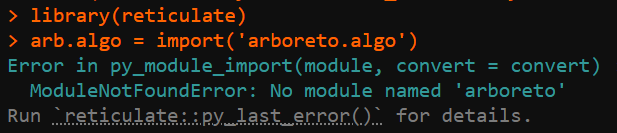
or dependency issues.
reticulate::use_python('/home/biomamba/.local/share/r-miniconda/envs/r-reticulate/bin/python') > arb.algo = import('arboreto.algo') Error in py_module_import(module, convert = convert) : ImportError: /usr/lib/x86_64-linux-gnu/libstdc++.so.6: version `GLIBCXX_3.4.29' not found (required by /home/biomamba/.local/share/r-miniconda/envs/r-reticulate/lib/python3.8/site-packages/pandas/_libs/window/aggregations.cpython-38-x86_64-linux-gnu.so) Run `reticulate::py_last_error()` for details.Or there are compatibility issues between R and Python data:
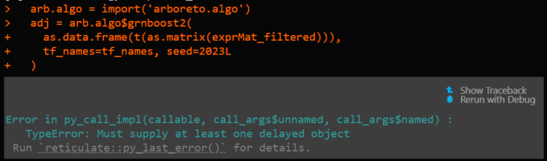
Therefore, the safest approach is to let R and Python work independently, that is, generate exprMat_filtered and export it locally, and complete the analysis in pure Python. The visualization highlights are as follows:
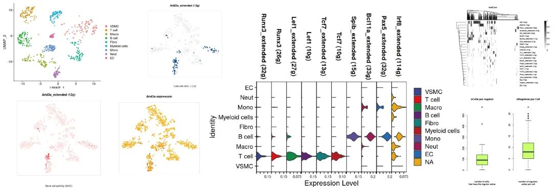
2. The R+Python Combination
If you have difficulty understanding the following content, you may want to study the:SCENIC single-cell transcription factor learning manual
This tutorial is demonstrated in a Linux environment using Rstudio. Those with insufficient computing resources can refer to:Environment for bioinformatics that supports your graduate studiesDedicated server, no need to seek help for bioinformatics analysis5090 is finally availableVisit link:https://biomamba.xiyoucloud.net/Welcome to contact customer service via WeChat [Biomamba_yunying] for assistance
1. Load R Packages
if (!requireNamespace("BiocManager", quietly =TRUE))install.packages("BiocManager")
BiocManager::version()
## [1] '3.20'# When your Bioconductor version is greater than 4.0
if(!require(SCENIC))BiocManager::install(c("AUCell", "RcisTarget"),ask = F,update = F);BiocManager::install(c("GENIE3"),ask = F,update = F)# These three packages are obviously essential to install
### Optional packages:
# AUCell dependency packages
if(!require(SCENIC))BiocManager::install(c("zoo", "mixtools", "rbokeh"),ask = F,update = F)
### t-SNEs computation dependency packages:
if(!require(SCENIC))BiocManager::install(c("DT", "NMF", "ComplexHeatmap", "R2HTML", "Rtsne"),ask = F,update = F)
# # These packages are used for parallel computation, unfortunately, they are not supported on Windows, so it is best to switch to Linux for large data calculations:
if(!require(SCENIC))BiocManager::install(c("doMC", "doRNG"),ask = F,update = F)
# Visualization output
# To export/visualize in http://scope.aertslab.org
if (!requireNamespace("devtools", quietly =TRUE))install.packages("devtools")
if(!require(SCopeLoomR))devtools::install_github("aertslab/SCopeLoomR", build_vignettes =TRUE)# SCopeLoomR is used to obtain test data
if (!requireNamespace("arrow", quietly =TRUE)) BiocManager::install('arrow')
# This package must be installed, otherwise an error will occur at runSCENIC_2_createRegulons, indicating that 'dbs' does not exist
library(SCENIC)# This has been installed, let's see if it can load normally
if(!require(SCENIC))devtools::install_github("aertslab/SCENIC")
packageVersion("SCENIC")# Here I installed version 1.3.1## [1] '1.3.1'library(SCENIC)
library(RcisTarget)
library(AUCell)
library(Seurat)2. Preprocessing in R
# Initialize SCENIC settings
data(list="motifAnnotations_mgi_v9", package="RcisTarget")
motifAnnotations_mgi <- motifAnnotations_mgi_v9
scenicOptions <-initializeScenic(org="mgi",# mouse fill 'mgi', human fill 'hgnc', fly fill 'dmel')
dbDir="./data/mouse.mm9/",
nCores=6)# Here you can set parallel computation
## Motif databases selected:
## mm9-500bp-upstream-7species.mc9nr.feather
## mm9-tss-centered-10kb-7species.mc9nr.feather## Using the column 'features' as feature index for the ranking database.
## Using the column 'features' as feature index for the ranking database.library(Seurat)
# Read test object
scRNA <-readRDS('./data/pbmcrenamed.rds')
# View test object dimensionality reduction plot:
DimPlot(scRNA) 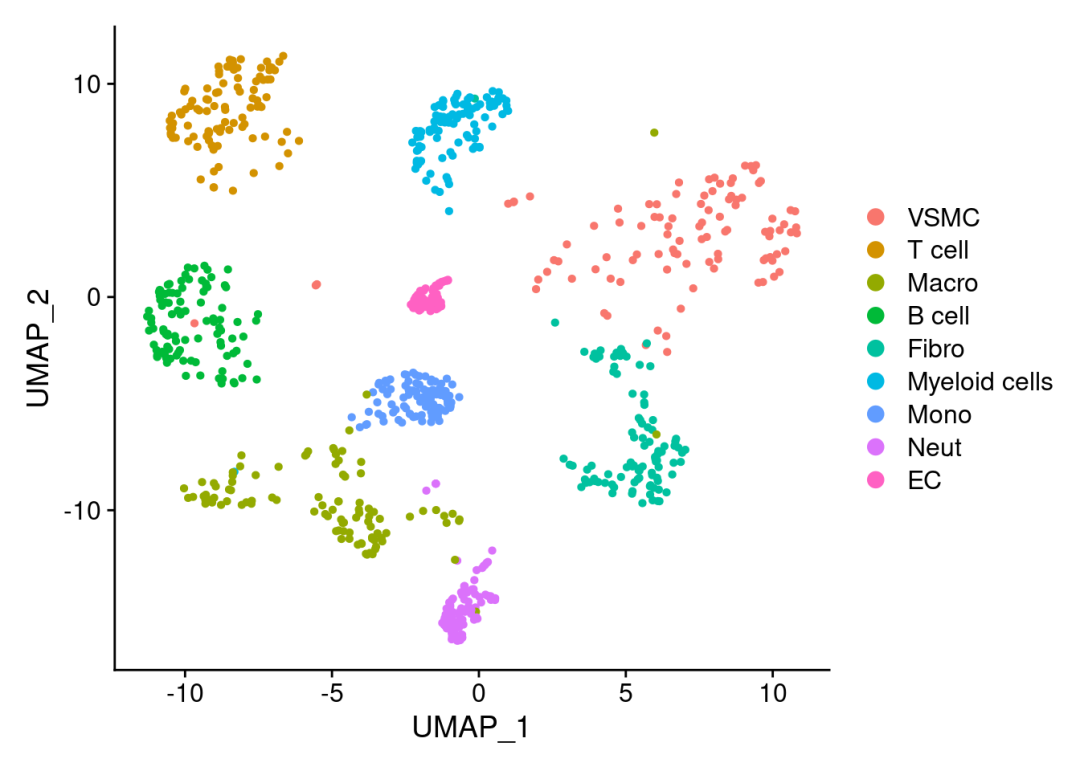
# Get expression matrix:
exprMat <-GetAssayData(scRNA ,'RNA','count')
# Convert to matrix object:
exprMat <-as.matrix(exprMat)
# Preliminary filtering of genes:
genesKept <-geneFiltering(exprMat, scenicOptions)
## Maximum value in the expression matrix: 26404## Ratio of detected vs non-detected: 0.12## Number of counts (in the dataset units) per gene:## Min. 1st Qu. Median Mean 3rd Qu. Max.
## 0.0 3.0 48.0 407.6 214.0 187278.0## Number of cells in which each gene is detected:## Min. 1st Qu. Median Mean 3rd Qu. Max.
## 0.00 3.00 39.00 99.42 143.00 897.00##
## Number of genes left after applying the following filters (sequential):## 11369 genes with counts per gene > 27## 11338 genes detected in more than 9 cells## Using the column 'features' as feature index for the ranking database.## 10021 genes available in RcisTarget database## Gene list saved in int/1.1_genesKept.RdsexprMat_filtered <- exprMat[genesKept, ]
# Calculate Spearman correlation:
runCorrelation(exprMat_filtered, scenicOptions)
# Take log:
exprMat_filtered_log <-log2(exprMat_filtered+1)
# Get TF names:
tf_names =getDbTfs(scenicOptions)
tf_names = Seurat::CaseMatch(
search = tf_names,
match =rownames(exprMat_filtered))
# Export expression matrix (needs to be transposed, as in Python, samples are usually rows and genes are columns) for subsequent Python reading:
write.csv(t(exprMat_filtered), file ="./data/expr_matrix_transposed.csv", row.names =TRUE)
# Export TF name list
write.csv(data.frame(tf_names = tf_names), file ="./data/tf_names.csv", row.names =FALSE)3. Complete in Python<span>grnboost</span>
### The following commands are executed in Python ###
import pandas as pd
from arboreto.algo import grnboost2

# Read R exported data
expr_matrix = pd.read_csv("data/expr_matrix_transposed.csv", index_col=0)
tf_names = pd.read_csv("data/tf_names.csv")["tf_names"].tolist()

# Ensure TF names exist in the expression matrix genes
available_genes = expr_matrix.columns.tolist()
tf_names = [tf for tf in tf_names if tf in available_genes]

# Run GRNBoost2
adj = grnboost2(
    expr_matrix,
    tf_names=tf_names,
    seed=2023,
    verbose=True
)

# Rename columns to match the expected format in R
adj.columns = ['TF', 'Target', 'weight']

# Save results (in CSV format readable by R)
adj.to_csv("data/grnboost2_results.csv", index=False)
The following is the running prompt information:
>>>### The following commands are executed in Python ###
>>>import pandas as pd
>>>from arboreto.algo import grnboost2
>>>
>>># Read R exported data
>>> expr_matrix = pd.read_csv("data/expr_matrix_transposed.csv", index_col=0)
>>> tf_names = pd.read_csv("data/tf_names.csv")["tf_names"].tolist()
>>>
>>># Ensure TF names exist in the expression matrix genes
>>> available_genes = expr_matrix.columns.tolist()
>>> tf_names = [tf for tf in tf_names if tf in available_genes]

>>>
>>># Run GRNBoost2
>>> adj = grnboost2(
...     expr_matrix,
...     tf_names=tf_names,
...     seed=2023,
...     verbose=True
... )
preparing dask client

parsing input
creating dask graph
19 partitions
computing dask graph
shutting down client and local cluster
finished
>>>
>>># Rename columns to match the expected format in R
>>> adj.columns = ['TF', 'Target', 'weight']
>>>
>>># Save results (in CSV format readable by R)
>>> adj.to_csv("data/grnboost2_results.csv", index=False)
4. Complete the Classic 4 Steps of SCENIC in R
Back to R:
# Read the GRN results output by Python
adj <-read.csv("data/grnboost2_results.csv")
# Convert to data frame and set column names (ensure consistency with previous format)
adj <-as.data.frame(adj)
colnames(adj) <-c('TF', 'Target', 'weight')

# Save as RDS file for subsequent analysis
saveRDS(adj, file =getIntName(scenicOptions, 'genie3ll'))

# Verify results
cat("Successfully read GRNBoost2 results, with a total of", nrow(adj), "regulatory relationships\n")

# Run the classic SCENIC steps 1-4
exprMat_log <-log2(exprMat+1)
scenicOptions@settings$dbs <- scenicOptions@settings$dbs["10kb"] # Toy run settings
scenicOptions <-runSCENIC_1_coexNetwork2modules(scenicOptions)

scenicOptions <-runSCENIC_2_createRegulons(scenicOptions, coexMethod=c("top5perTarget")) # Toy run settings
scenicOptions <-runSCENIC_3_scoreCells(scenicOptions, exprMat_log)

scenicOptions <-runSCENIC_4_aucell_binarize(scenicOptions)# Binarize the AUCell matrix

# Save the image
save.image('data/biomamba_scenic.rdata')
# At this point, we have the same project files as executing SCENIC purely in R:
tree ./int## [01;34m./int[00m
## ├── 1.1_genesKept.Rds
## ├── 1.2_corrMat.Rds
## ├── 1.4_GENIE3_linkList.Rds
## ├── 1.5_weightPlot.pdf
## ├── 1.6_tfModules_asDF.Rds
## ├── 2.1_tfModules_forMotifEnrichmet.Rds
## ├── 2.2_motifs_AUC.Rds
## ├── 2.3_motifEnrichment.Rds
## ├── 2.4_motifEnrichment_selfMotifs_wGenes.Rds
## ├── 2.5_regulonTargetsInfo.Rds
## ├── 2.6_regulons_asGeneSet.Rds
## ├── 2.6_regulons_asIncidMat.Rds
## ├── 3.1_regulons_forAUCell.Rds
## ├── 3.2_aucellGenesStats.pdf
## ├── 3.3_aucellRankings.Rds
## ├── 3.4_regulonAUC.Rds
## ├── 3.5_AUCellThresholds_Info.tsv
## ├── 3.5_AUCellThresholds.Rds
## ├── 4.1_binaryRegulonActivity.Rds
## ├── 4.2_binaryRegulonActivity_nonDupl.Rds
## ├── 4.3_regulonSelections.Rds
## ├── 4.4_binaryRegulonOrder.Rds
## └── tSNE_AUC_50pcs_30perpl.Rds
##
## 0 directories, 23 files# Read AUCell Score matrix:
auc_score <-getAUC(readRDS("int/3.4_regulonAUC.Rds"))
# Add to annotation information:
scRNA <-AddMetaData(scRNA,metadata =t(auc_score))
# Violin plot for a few transcription factors:
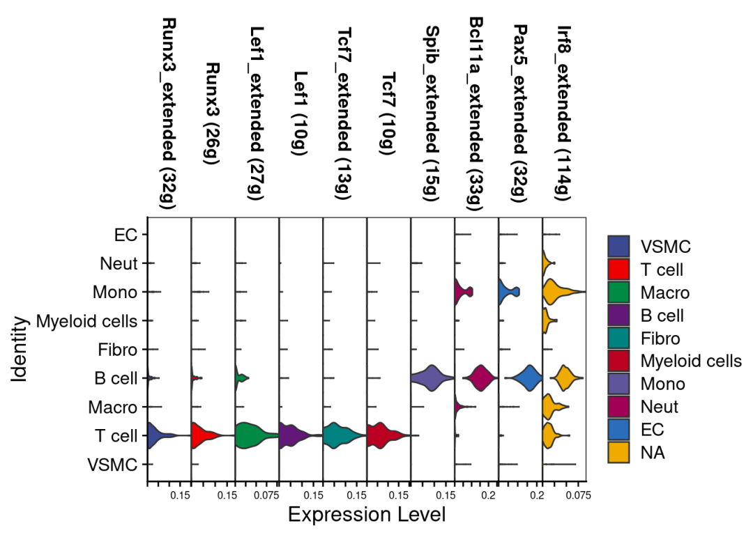
VlnPlot(scRNA,rownames(auc_score)[1:10],stack = T,
cols =c(ggsci::pal_aaas()(8),ggsci::pal_bmj()(8))
)
More visualizations can be seen in:SCENIC single-cell transcription factor learning manualSCENIC single-cell transcription factor downstream explorationSCENIC transcription factor regulatory network diagram
3. Test Files and Demonstration Environment
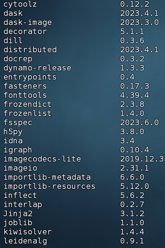
Any tutorial that does not provide test files and analysis environment versions is untrustworthy. The code and test files provided in this post can be downloaded from the following link:
Files shared via cloud storage: R and Python combined analysis SCENIC process
Link: https://pan.baidu.com/s/1DQdzV7QzuwJ89-Cs7xsnmQ?pwd=tfdx
Extraction code: tfdx

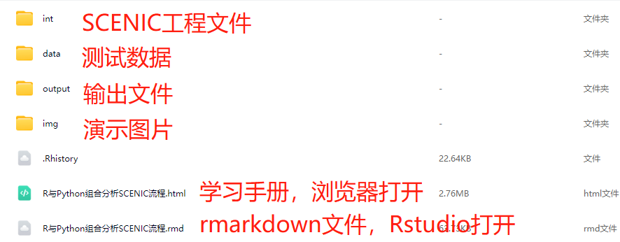 R language demonstration environment:
sessionInfo()## R version 4.4.2 (2024-10-31)
## Platform: x86_64-pc-linux-gnu
## Running under: Ubuntu 20.04.4 LTS
##
## Matrix products: default
## BLAS: /usr/lib/x86_64-linux-gnu/openblas-pthread/libblas.so.3
## LAPACK: /usr/lib/x86_64-linux-gnu/openblas-pthread/liblapack.so.3; LAPACK version 3.9.0
##
## locale:
## [1] LC_CTYPE=en_US.UTF-8 LC_NUMERIC=C
## [3] LC_TIME=en_US.UTF-8 LC_COLLATE=en_US.UTF-8
## [5] LC_MONETARY=en_US.UTF-8 LC_MESSAGES=en_US.UTF-8
## [7] LC_PAPER=en_US.UTF-8 LC_NAME=C
## [9] LC_ADDRESS=C LC_TELEPHONE=C
## [11] LC_MEASUREMENT=en_US.UTF-8 LC_IDENTIFICATION=C
##
## time zone: Etc/UTC
## tzcode source: system (glibc)
##
## attached base packages:
## [1] stats graphics grDevices utils datasets methods base
##
## other attached packages:
## [1] Seurat_5.2.1 SeuratObject_5.0.2 sp_2.2-0 AUCell_1.28.0
## [5] RcisTarget_1.26.0 SCopeLoomR_0.13.0 SCENIC_1.3.1
##
## loaded via a namespace (and not attached):
## [1] RcppAnnoy_0.0.22 splines_4.4.2
## [3] later_1.4.1 bitops_1.0-9
## [5] tibble_3.2.1 R.oo_1.27.0
## [7] polyclip_1.10-7 graph_1.84.1
## [9] XML_3.99-0.18 fastDummies_1.7.5
## [11] lifecycle_1.0.4 globals_0.16.3
## [13] lattice_0.22-6 hdf5r_1.3.12
## [15] MASS_7.3-64 magrittr_2.0.3
## [17] plotly_4.10.4 sass_0.4.9
## [19] rmarkdown_2.29 jquerylib_0.1.4
## [21] yaml_2.3.10 remotes_2.5.0
## [23] httpuv_1.6.15 sctransform_0.4.1
## [25] spam_2.11-1 spatstat.sparse_3.1-0
## [27] sessioninfo_1.2.2 pkgbuild_1.4.6
## [29] reticulate_1.43.0.9001 cowplot_1.1.3
## [31] pbapply_1.7-2 DBI_1.2.3
## [33] RColorBrewer_1.1-3 abind_1.4-8
## [35] pkgload_1.4.0 zlibbioc_1.52.0
## [37] Rtsne_0.17 GenomicRanges_1.58.0
## [39] purrr_1.0.2 R.utils_2.12.3
## [41] BiocGenerics_0.52.0 RCurl_1.98-1.16
## [43] GenomeInfoDbData_1.2.13 IRanges_2.40.1
## [45] S4Vectors_0.44.0 ggrepel_0.9.6
## [47] irlba_2.3.5.1 spatstat.utils_3.1-4
## [49] listenv_0.9.1 openintro_2.5.0
## [51] goftest_1.2-3 airports_0.1.0
## [53] RSpectra_0.16-2 spatstat.random_3.4-1
## [55] annotate_1.84.0 fitdistrplus_1.2-2
## [57] parallelly_1.42.0 DelayedMatrixStats_1.28.1
## [59] codetools_0.2-20 DelayedArray_0.32.0
## [61] tidyselect_1.2.1 UCSC.utils_1.2.0
## [63] farver_2.1.2 spatstat.explore_3.4-3
## [65] matrixStats_1.5.0 stats4_4.4.2
## [67] jsonlite_1.8.9 ellipsis_0.3.2
## [69] progressr_0.15.1 ggridges_0.5.6
## [71] survival_3.8-3 tools_4.4.2
## [73] ica_1.0-3 Rcpp_1.0.14
## [75] glue_1.8.0 gridExtra_2.3
## [77] SparseArray_1.6.0 xfun_0.50
## [79] MatrixGenerics_1.18.1 usethis_3.1.0
## [81] GenomeInfoDb_1.42.1 dplyr_1.1.4
## [83] withr_3.0.2 BiocManager_1.30.25
## [85] fastmap_1.2.0 digest_0.6.37
## [87] R6_2.5.1 mime_0.12
## [89] colorspace_2.1-1 scattermore_1.2
## [91] tensor_1.5 spatstat.data_3.1-6
## [93] RSQLite_2.3.9 R.methodsS3_1.8.2
## [95] ggsci_3.2.0 tidyr_1.3.1
## [97] generics_0.1.3 data.table_1.16.4
## [99] usdata_0.3.1 httr_1.4.7
## [101] htmlwidgets_1.6.4 S4Arrays_1.6.0
## [103] uwot_0.2.2 pkgconfig_2.0.3
## [105] gtable_0.3.6 blob_1.2.4
## [107] lmtest_0.9-40 XVector_0.46.0
## [109] htmltools_0.5.8.1 profvis_0.4.0
## [111] dotCall64_1.2 GSEABase_1.64.0
## [113] scales_1.3.0 Biobase_2.66.0
## [115] png_0.1-8 spatstat.univar_3.1-3
## [117] knitr_1.49 rstudioapi_0.17.1
## [119] reshape2_1.4.4 tzdb_0.4.0
## [121] nlme_3.1-168 cachem_1.1.0
## [123] zoo_1.8-12 stringr_1.5.1
## [125] KernSmooth_2.23-26 parallel_4.4.2
## [127] miniUI_0.1.1.1 arrow_18.1.0.1
## [129] AnnotationDbi_1.68.0 pillar_1.10.1
## [131] grid_4.4.2 vctrs_0.6.5
## [133] RANN_2.6.2 urlchecker_1.0.1
## [135] promises_1.3.2 xtable_1.8-4
## [137] cluster_2.1.8 evaluate_1.0.3
## [139] readr_2.1.5 cli_3.6.3
## [141] compiler_4.4.2 rlang_1.1.5
## [143] crayon_1.5.3 future.apply_1.11.3
## [145] labeling_0.4.3 plyr_1.8.9
## [147] fs_1.6.5 stringi_1.8.4
## [149] deldir_2.0-4 viridisLite_0.4.2
## [151] assertthat_0.2.1 munsell_0.5.1
## [153] Biostrings_2.74.1 lazyeval_0.2.2
## [155] spatstat.geom_3.4-1 devtools_2.4.5
## [157] Matrix_1.7-2 RcppHNSW_0.6.0
## [159] hms_1.1.3 patchwork_1.3.0
## [161] sparseMatrixStats_1.18.0 bit64_4.6.0-1
## [163] future_1.34.0 ggplot2_3.5.1
## [165] KEGGREST_1.46.0 shiny_1.10.0
## [167] SummarizedExperiment_1.36.0 ROCR_1.0-11
## [169] igraph_2.1.4 memoise_2.0.1
## [171] bslib_0.9.0 bit_4.5.0.1
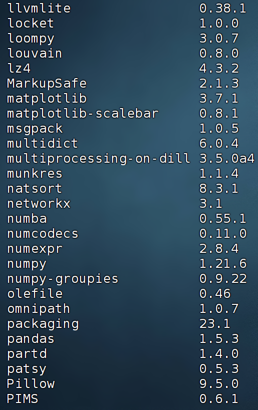
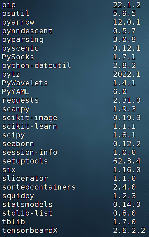
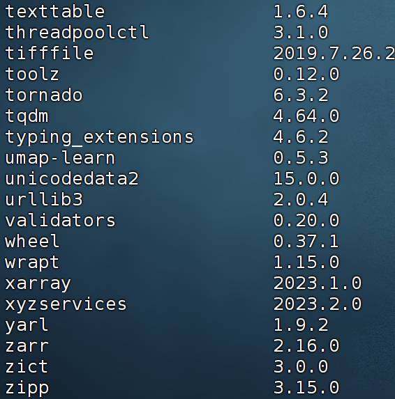
## [173] cherryblossom_0.1.0Python environment: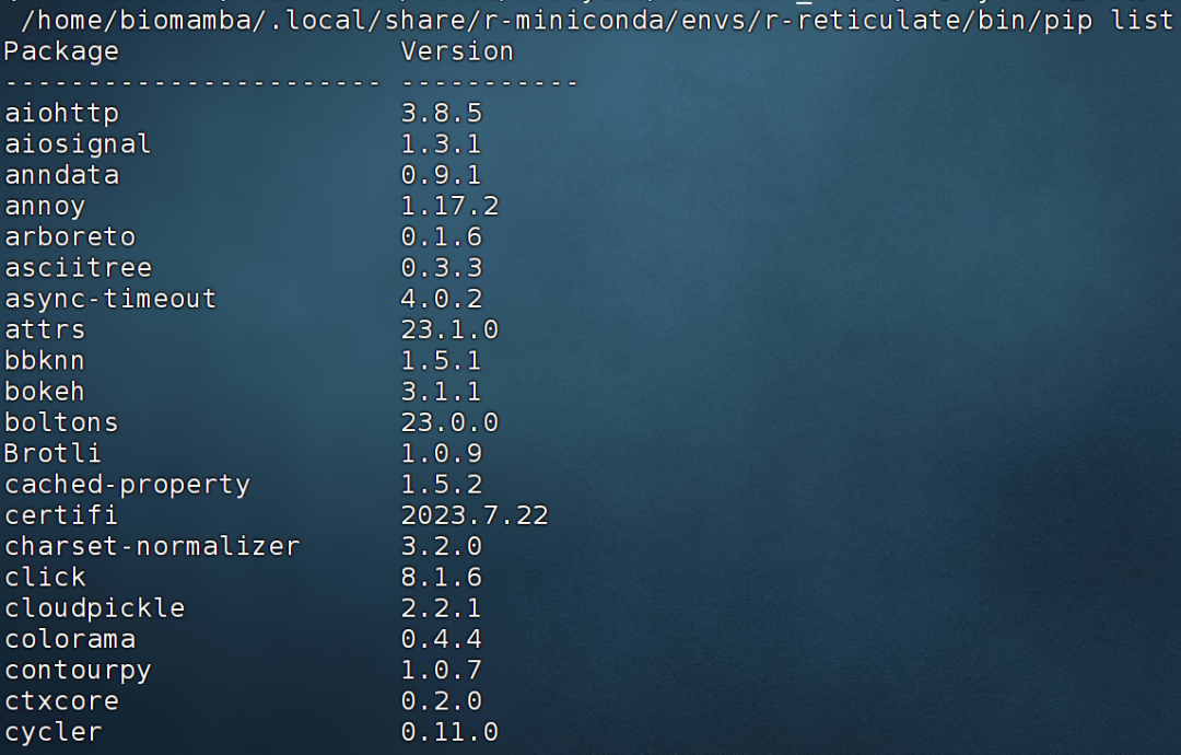

How to Contact Us

 Leave a message to receive materials, an out-of-the-box single-cell analysis image via WeChat [Biomamba_yunying], making it convenient for everyone to communicate at any time. We have also built a group chat matrix, and everyone is welcome to join the discussion.After reading these articles, you can add tips for beginners in bioinformatics without searching, you have no right to speak
Students who already have contact information for the bioinformatics basedo not need to add again

 Every like and view you give, I take seriously as appreciation