Skyborn

Lightning-Fast Trend Calculation

In climate science and earth science research, calculating time trends from large-scale grid data is a common and important task. Traditional methods often require looping through each grid point, which is inefficient. The Skyborn library enhances the efficiency of trend analysis through vectorized computations.

Github:<span>https://github.com/QianyeSu/Skyborn</span>

Performance Comparison

Performance tests were conducted using GPCP precipitation data (1979-2014, 36 years × 72×144 grid points = 10,368 locations) with four methods:

Method	Computation Time	Speedup Relative to Skyborn
Skyborn Linear Regression	0.014 seconds	Baseline
Scipy Linear Regression	3.619 seconds	258.3 times slower
Skyborn Mann-Kendall	0.494 seconds	Baseline
PyMannKendall	13.625 seconds	27.6 times slower

Core Advantages

1. Exceptional Computational Performance

• Linear Regression: 258 times faster than traditional scipy methods
• Mann-Kendall Test: 28 times faster than PyMannKendall
• Vectorized computations fully utilize modern CPU performance

2. Consistent Computational Results

Test results show that Skyborn is numerically consistent with traditional methods:

• Skyborn vs Scipy Linear Regression:Difference is 0
• Skyborn vs PyMannKendall:Difference is 0
• Ensures accuracy and reliability in scientific computations

3. Simple and User-Friendly API

from skyborn.calc import linear_regression, mann_kendall_multidim

# Linear trend analysis - one line of code
trend, p_values = linear_regression(data_3d, time_series)

# Mann-Kendall non-parametric trend test
mk_result = mann_kendall_multidim(data_3d, axis=0)
trend = mk_result['trend']
p_values = mk_result['p']

Practical Application Case

Global Precipitation Trend Analysis (1979-2014)

Using 36 years of GPCP precipitation data, the results show:

Trend Distribution:

• Positive trend area: 51.0% (precipitation increase)
• Negative trend area: 49.0% (precipitation decrease)
• Statistically significant area: 32.8% (p < 0.05)

Extremes:

• Maximum increasing trend: +7.6 × 10⁻² mm/day/year
• Maximum decreasing trend: -13.1 × 10⁻² mm/day/year

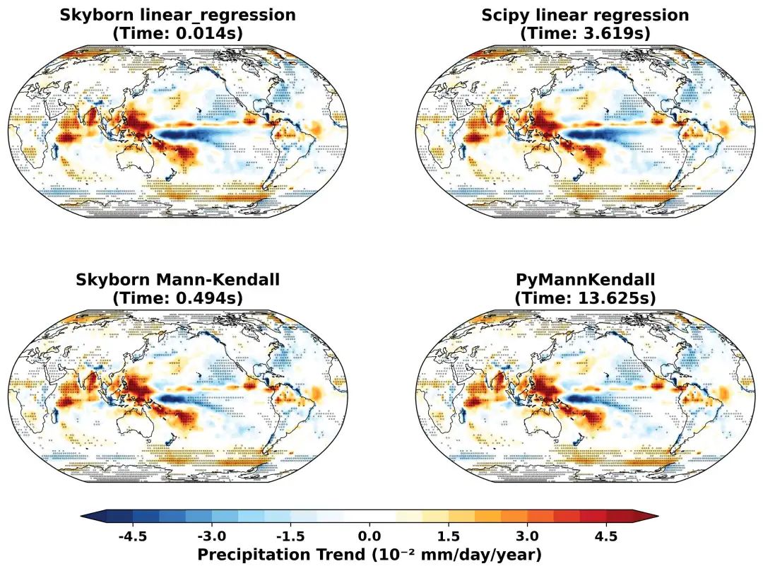
Figure: Comparison of global precipitation trends calculated by four methods, with black dots indicating statistically significant areas (p < 0.05)

💡 Method Comparison

Linear Regression vs Mann-Kendall

• Linear Regression: Suitable for linear trends, sensitive to outliers
• Mann-Kendall: Non-parametric method, robust to outliers, suitable for non-linear trends. For more on Mann-Kendall, see previous articles ——— Python | Why Choose Mann-Kendall Trend Test?
• Difference in trends between the two methods: RMS = 0.28 × 10⁻² mm/day/year,

Technical Features

Vectorized Computing Architecture

• Optimized based on NumPy and SciKit-learn
• Avoids Python loops, reducing code
• High memory efficiency, supports large-scale data processing

Statistical Significance Testing

• Automatically calculates p-values, supports multiple testing

Easy Installation

Environment Requirements: Python 3.9-2.12

Platform: Linux, Windows, Mac (supports both Intel CPU and Apple Silicon chips)

pip install skyborn

Plotting Code

# -*- coding: utf-8 -*-
"""
GPCP Precipitation Trend Analysis (1979-2014)
Comparison of trend calculation methods and spatial visualization

@author: Skyborn
"""
from scipy import stats
import numpy as np
import matplotlib.pyplot as plt
import xarray as xr
import cartopy.crs as ccrs
import cartopy.feature as cfeature
from skyborn.calc import mann_kendall_multidim, linear_regression
import cmaps
import pymannkendall as pmk
import time

data = xr.open_dataset(r"precip.mon.mean.nc").sel(
    time=slice("1979", "2014")).groupby("time.year").mean("time")

pr = data.precip.values  # Shape: (years, lat, lon)
year = data.year.values
lat = data.lat.values
lon = data.lon.values

start_time = time.time()
pr_trend_skyborn, p_values_skyborn = linear_regression(pr, year)
time_skyborn = time.time() - start_time
start_time = time.time()
pr_trend_scipy = np.zeros((len(lat), len(lon)))
p_values_scipy = np.zeros((len(lat), len(lon)))

for i in range(len(lat)):
    for j in range(len(lon)):
        if np.isfinite(pr[:, i, j]).all():
            slope, intercept, r_value, p_value, std_err = stats.linregress(
                year, pr[:, i, j])
            pr_trend_scipy[i, j] = slope
            p_values_scipy[i, j] = p_value
        else:
            pr_trend_scipy[i, j] = np.nan
            p_values_scipy[i, j] = np.nan
            
time_scipy = time.time() - start_time
start_time = time.time()
mk_result = mann_kendall_multidim(pr, axis=0)
pr_trend_mk_skyborn = mk_result['trend']
p_values_mk_skyborn = mk_result['p']
time_mk_skyborn = time.time() - start_time

start_time = time.time()
pr_trend_pmk = np.zeros((len(lat), len(lon)))
p_values_pmk = np.zeros((len(lat), len(lon)))

for i in range(len(lat)):
    for j in range(len(lon)):
        if np.isfinite(pr[:, i, j]).all():
            result = pmk.original_test(pr[:, i, j])
            pr_trend_pmk[i, j] = result.slope
            p_values_pmk[i, j] = result.p
        else:
            pr_trend_pmk[i, j] = np.nan
            p_values_pmk[i, j] = np.nan
time_pmk = time.time() - start_time

pr_trend_skyborn_mmyr = pr_trend_skyborn * 100
pr_trend_scipy_mmyr = pr_trend_scipy * 100
pr_trend_mk_skyborn_mmyr = pr_trend_mk_skyborn * 100
pr_trend_pmk_mmyr = pr_trend_pmk * 100


fig = plt.figure(figsize=(12, 8))

all_trends = [pr_trend_skyborn_mmyr, pr_trend_scipy_mmyr,
              pr_trend_mk_skyborn_mmyr, pr_trend_pmk_mmyr]

trend_max = 5
cmap = cmaps.BlueWhiteOrangeRed
norm = plt.Normalize(vmin=-trend_max, vmax=trend_max)


ax1 = plt.subplot(2, 2, 1, projection=ccrs.Robinson(central_longitude=180))
ax1.set_global()
ax1.add_feature(cfeature.COASTLINE, linewidth=0.5)
ax1.add_feature(cfeature.OCEAN, color='lightgray', alpha=0.5)

im1 = ax1.contourf(lon, lat, pr_trend_skyborn_mmyr,
                   levels=np.linspace(-trend_max, trend_max, 21),
                   cmap=cmap, norm=norm, transform=ccrs.PlateCarree(), extend='both')

lon_sig, lat_sig = np.meshgrid(lon, lat)
sig_mask = p_values_skyborn < 0.05
ax1.scatter(lon_sig[sig_mask], lat_sig[sig_mask], s=0.1, c='black', alpha=0.6, transform=ccrs.PlateCarree())
ax1.set_title(
    f'Skyborn linear_regression\n(Time: {time_skyborn:.3f}s)', fontweight='bold')


ax2 = plt.subplot(2, 2, 2, projection=ccrs.Robinson(central_longitude=180))
ax2.set_global()
ax2.add_feature(cfeature.COASTLINE, linewidth=0.5)
ax2.add_feature(cfeature.OCEAN, color='lightgray', alpha=0.5)

im2 = ax2.contourf(lon, lat, pr_trend_scipy_mmyr,
                   levels=np.linspace(-trend_max, trend_max, 21),
                   cmap=cmap, norm=norm, transform=ccrs.PlateCarree(), extend='both')

sig_mask2 = p_values_scipy < 0.05
ax2.scatter(lon_sig[sig_mask2], lat_sig[sig_mask2], s=0.1, c='black', alpha=0.6, transform=ccrs.PlateCarree())
ax2.set_title(
    f'Scipy linear regression\n(Time: {time_scipy:.3f}s)', fontweight='bold')


ax3 = plt.subplot(2, 2, 3, projection=ccrs.Robinson(central_longitude=180))
ax3.set_global()
ax3.add_feature(cfeature.COASTLINE, linewidth=0.5)
ax3.add_feature(cfeature.OCEAN, color='lightgray', alpha=0.5)

im3 = ax3.contourf(lon, lat, pr_trend_mk_skyborn_mmyr,
                   levels=np.linspace(-trend_max, trend_max, 21),
                   cmap=cmap, norm=norm, transform=ccrs.PlateCarree(), extend='both')

sig_mask3 = p_values_mk_skyborn < 0.05
ax3.scatter(lon_sig[sig_mask3], lat_sig[sig_mask3], s=0.1, c='black', alpha=0.6, transform=ccrs.PlateCarree())
ax3.set_title(
    f'Skyborn Mann-Kendall\n(Time: {time_mk_skyborn:.3f}s)', fontweight='bold')

ax4 = plt.subplot(2, 2, 4, projection=ccrs.Robinson(central_longitude=180))
ax4.set_global()
ax4.add_feature(cfeature.COASTLINE, linewidth=0.5)
ax4.add_feature(cfeature.OCEAN, color='lightgray', alpha=0.5)

im4 = ax4.contourf(lon, lat, pr_trend_pmk_mmyr,
                   levels=np.linspace(-trend_max, trend_max, 21),
                   cmap=cmap, norm=norm, transform=ccrs.PlateCarree(), extend='both')

sig_mask4 = p_values_pmk < 0.05
ax4.scatter(lon_sig[sig_mask4], lat_sig[sig_mask4], s=0.1, c='black', alpha=0.6, transform=ccrs.PlateCarree())
ax4.set_title(f'PyMannKendall\n(Time: {time_pmk:.3f}s)', fontweight='bold')


cbar_ax = fig.add_axes([0.2, 0.1, 0.6, 0.02])  # [left, bottom, width, height]
cbar = plt.colorbar(im1, cax=cbar_ax, orientation='horizontal', extend='both')
cbar.set_label('Precipitation Trend (10⁻² mm/day/year)', fontweight='bold', fontsize=14)

plt.show()

Applicable Scenarios

Suitable for trend analysis that requires processinglarge-scale multidimensional arrays and high-density grid data:

• Large-scale climate data: Global/Regional climate model outputs (thousands to millions of grid points)
• High-resolution remote sensing data: Satellite image time series (Landsat, MODIS, Sentinel, etc.)
• Dense observation networks: Long time series from meteorological station networks, ocean buoy arrays
• Multidimensional Earth science data: Temporal and spatial trends of three-dimensional ocean data, atmospheric profile data
• Big data environmental monitoring: Air quality grid data, water quality monitoring networks
• Batch time series processing: When you need to analyze thousands of time series simultaneously

Performance advantages become more pronounced with larger data volumes:

• Number of grid points > 1000: Significant acceleration
• Number of grid points > 10000:Acceleration of over a hundred times

Conclusion

The Skyborn library redefines the efficiency standard for spatial trend analysis through vectorized computations, achieving speed improvements of dozens to hundreds of times while ensuring computational accuracy.

For more information, please visit: Skyborn Documentation ———<span>https://skyborn.readthedocs.io/en/latest/</span>

Previous Articles

• Python | MJO | Phase Diagram
• Python | Longitude Conversion Between Hemispheres
• Python | Atmospheric Science | Partial Correlation
• Python | Meteorological Plotting | Typhoon Precipitation
• Python | Resolving cmaps Library Errors
• Python | Batch Downloading NCEP2 Reanalysis Data
• Python | North Atlantic Oscillation | NAO Index | EOF