1. Overview
1.1 Robot Control System
The robot control system is the brain of the robot and is the main factor determining the robot’s functions and performance. The primary task of industrial robot control technology is to control the motion position, posture, trajectory, operation sequence, and timing of actions of industrial robots within their workspace. It features simple programming, software menu operations, a user-friendly human-machine interface, online operation prompts, and ease of use.
1.2 Key Technologies in Robot Control
The key technologies include:
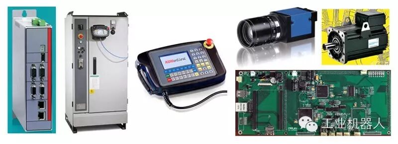
(1)Open modular control system architecture: It adopts a distributed CPU computer structure, divided into robot controllers (RC), motion controllers (MC), opto-isolated I/O control boards, sensor processing boards, and programming teaching boxes. The robot controller (RC) and programming teaching box communicate via serial/CAN bus. The main computer of the robot controller (RC) completes motion planning, interpolation, position servo, main control logic, digital I/O, sensor processing, etc., while the programming teaching box displays information and inputs commands.
(2)Modular hierarchical controller software system: The software system is built on an open-source real-time multitasking operating system, Linux, and is designed with a layered and modular structure to achieve software system openness. The entire controller software system is divided into three levels: hardware driver layer, core layer, and application layer. Each level addresses different functional requirements and corresponds to different levels of development, with each level composed of several functionally opposing modules that collaborate to achieve the functions provided by that level.
(3)Robot fault diagnosis and safety maintenance technology: Diagnosing robot faults through various information and performing corresponding maintenance is a key technology to ensure the safety of robots.
(4)Networked robot controller technology: Currently, the application of robots is evolving from single robot workstations to robot production lines, making the networking technology of robot controllers increasingly important. The controller features serial, fieldbus, and Ethernet networking capabilities, facilitating communication between robot controllers and between robot controllers and host computers, which aids in monitoring, diagnosing, and managing robot production lines.
2. PID Control in Robotics
2.1 Components of a PID Controller
A PID controller consists of a proportional unit (P), an integral unit (I), and a derivative unit (D). The relationship between the input e(t) and output u(t) is given by u(t) = Kp(e(t) + (1/TI)∫e(t)dt + TD*de(t)/dt
The limits of integration are 0 and t, thus its transfer function is:G(s) = U(s)/E(s) = Kp(1 + 1/(TI*s) + TD*s); where Kp is the proportional coefficient; TI is the integral time constant; and TD is the derivative time constant.
Due to its wide applicability and flexible use, there are already standardized products available, where only three parameters (Kp, Ti, and Td) need to be set during use. In many cases, not all three units are necessary; one or two units can be used, but the proportional control unit is essential.
Firstly, PID has a wide range of applications. Although many industrial processes are nonlinear or time-varying, they can be simplified into basic linear systems with dynamic characteristics that do not change over time, allowing PID to control them.
Secondly, PID parameters are relatively easy to tune. That is, the PID parameters Kp, Ti, and Td can be tuned in a timely manner according to the dynamic characteristics of the process. If the dynamic characteristics of the process change, for example, due to load changes, the PID parameters can be retuned.

2.2 Current Research Status of PID Controllers
Despite these drawbacks, PID controllers are the simplest and sometimes the best controllers.
Currently, the level of industrial automation has become an important indicator of modernization across various industries. At the same time, the development of control theory has gone through three stages: classical control theory, modern control theory, and intelligent control theory. A typical example of intelligent control is fuzzy fully automatic washing machines. Automatic control systems can be divided into open-loop control systems and closed-loop control systems. A control system includes controllers, sensors, transmitters, actuators, and input-output interfaces. The output of the controller is applied to the controlled system through the output interface and actuator; the controlled variable of the control system is sent to the controller through the sensor and transmitter via the input interface. Different control systems have different sensors, transmitters, and actuators. For example, a pressure control system requires a pressure sensor. The sensor for an electric heating control system is a temperature sensor. Currently, PID control and its controllers or intelligent PID controllers (instruments) have been widely applied in engineering practice, with various PID controller products developed by major companies featuring automatic tuning capabilities for PID parameters, where the automatic adjustment of PID controller parameters is achieved through intelligent adjustment or self-calibration and adaptive algorithms.
2.3 Limitations of PID Controllers
In some cases, PID controllers designed for specific systems perform well, but they still have some issues that need to be addressed:
If self-tuning is model-based, it is challenging to find and maintain a good process model for the retuning of PID parameters online. During closed-loop operation, it requires inserting a test signal into the process. This method can cause disturbances, so model-based PID parameter self-tuning is not very effective in industrial applications.
If self-tuning is based on control laws, it is often difficult to distinguish between the effects caused by load disturbances and those caused by changes in process dynamics, leading to overshoot due to the influence of disturbances, resulting in unnecessary adaptive transitions. Additionally, due to the lack of mature stability analysis methods for control law-based systems, there are many issues regarding the reliability of parameter tuning.
Therefore, many self-tuning PID controllers often operate in automatic tuning mode rather than continuous self-tuning mode. Automatic tuning typically refers to the automatic calculation of PID parameters based on a simple process model determined from open-loop conditions.
PID does not perform well in controlling complex processes that are nonlinear, time-varying, coupled, and have uncertain parameters and structures. Most importantly, if a PID controller cannot control a complex process, no parameter tuning will help.
3. Principles and Characteristics of PID Control
3.1 Principles of PID Control
In practical engineering, the most widely used control law for regulators is proportional, integral, and derivative control, referred to as PID control, also known as PID regulation. The PID controller has been around for nearly 70 years, and its simple structure, good stability, reliability, and ease of adjustment have made it one of the main technologies in industrial control. When the structure and parameters of the controlled object cannot be fully grasped, or when an accurate mathematical model cannot be obtained, and other control theory techniques are difficult to apply, the structure and parameters of the system controller must rely on experience and field debugging to determine, making PID control technology the most convenient option. That is, when we do not fully understand a system and the controlled object, or cannot obtain system parameters through effective measurement methods, PID control technology is the most suitable. In practice, there are also PI and PD controls. The PID controller calculates the control quantity based on the system’s error using proportional, integral, and derivative calculations.
Proportional (P) Control
Proportional control is the simplest form of control. The output of its controller is proportional to the input error signal. When only proportional control is used, the system output has a steady-state error.
Integral (I) Control
In integral control, the output of the controller is proportional to the integral of the input error signal. For an automatic control system, if there is a steady-state error after reaching steady state, it is said that this control system has a steady-state error or is simply a non-zero system. To eliminate steady-state error, an integral term must be introduced into the controller. The integral term depends on the time integral of the error, and as time increases, the integral term will grow. Thus, even if the error is small, the integral term will increase over time, pushing the controller’s output to increase, further reducing the steady-state error until it equals zero. Therefore, a proportional + integral (PI) controller can ensure that the system has no steady-state error after reaching steady state.
Derivative (D) Control
In derivative control, the output of the controller is proportional to the derivative of the input error signal (i.e., the rate of change of the error). During the adjustment process of an automatic control system to overcome errors, oscillations or even instability may occur. This is due to the presence of significant inertia elements or lag components that suppress the error, with their changes always lagging behind the changes in the error. The solution is to make the change in the suppression of the error lead, meaning that when the error approaches zero, the suppression of the error should also be zero. This means that introducing only the proportional term in the controller is often insufficient; the role of the proportional term is merely to amplify the magnitude of the error, while what is needed now is to add the derivative term, which can predict the trend of error changes. Thus, a proportional + derivative control (PD) controller can preemptively make the suppression of the error control action equal to zero or even negative, thereby avoiding severe overshoot of the controlled quantity. Therefore, for controlled objects with significant inertia or lag, a proportional + derivative (PD) controller can improve the dynamic characteristics of the system during the adjustment process.
3.2 Characteristics of PID Control
In PID control, the characteristic of integral control is that as long as there is still a residual error (i.e., the remaining control deviation), integral control gradually increases the control action until the residual error disappears. Therefore, the effect of integration is relatively slow; except in special cases, as a basic control action, it cannot respond quickly. The characteristic of derivative control is that although the actual measured value is still lower than the set value, its rapid upward momentum needs to be suppressed early; otherwise, it will be too late to react when the actual value exceeds the set value. This is where derivative control comes into play. As a basic control action, derivative control only looks at the trend, not the specific value, so the ideal situation is to stabilize the actual value, but where it stabilizes depends on luck, so derivative control cannot serve as a basic control action. Proportional control does not have these issues; it reacts quickly, has good stability, and is the most fundamental control action, referred to as the “skin”; integral and derivative controls enhance the effect of proportional control and are rarely used alone, hence referred to as the “fur.” In practical use, proportional and integral controls are generally used together, with proportional control taking the main control action and integral control helping to eliminate residual errors. Derivative control is only adopted when the controlled object reacts slowly and needs to respond early to compensate.
4. Tuning Parameters of PID Controllers
The tuning of PID controller parameters is the core content of control system design. It determines the values of the proportional coefficient, integral time, and derivative time of the PID controller based on the characteristics of the controlled process. There are many methods for tuning PID controller parameters, which can be broadly categorized into two types: theoretical calculation tuning methods and engineering tuning methods. The theoretical calculation tuning method mainly relies on the mathematical model of the system to determine the controller parameters through theoretical calculations. The data obtained from this method may not be directly usable and must be adjusted and modified through engineering practice. The engineering tuning method mainly relies on engineering experience and is conducted directly in the experiments of the control system, with simple methods that are easy to master and widely adopted in engineering practice. The engineering tuning methods for PID controller parameters mainly include the critical ratio method, reaction curve method, and decay method. Each of these methods has its characteristics, but they all share the common point of tuning controller parameters through experiments and then applying engineering experience formulas. However, regardless of which method is used to obtain the controller parameters, final adjustments and improvements must be made during actual operation. Currently, the critical ratio method is commonly used. The steps for tuning PID controller parameters using this method are as follows: (1) First, pre-select a sufficiently short sampling period for the system to operate; (2) Only add the proportional control element until the system exhibits critical oscillation in response to a step input, recording the proportional gain and critical oscillation period at this time; (3) Calculate the PID controller parameters using formulas under certain control conditions.
The robot control system is the brain of the robot and is the main factor determining the robot’s functions and performance. The robot controller is a device that controls the robot to complete specific actions or tasks based on commands and sensor information; it is the heart of the robot, determining the quality of the robot’s performance. Robotics technology involves multiple disciplines, including computer science, electronics, and control, and has become an important field and research hotspot in the development of high-tech in recent years. With the development of robotics technology and the continuous expansion of application fields, higher performance requirements are placed on robots. Therefore, how to effectively apply research results from other fields (such as image processing, voice recognition, optimal control, artificial intelligence, etc.) to the real-time operation of robot control systems is a challenging research task. The research on modular, standardized robot controllers with an open structure undoubtedly has significant implications for improving robot performance and autonomy, as well as promoting the development of robotics technology.