1. Plotting Command
plot(x,y)
If x and y are vectors of equal length, it plots a 2D curve with x and y as the horizontal and vertical axes;
plot(x1,y1,x2,y2,…)
In this format, each pair of x and y must meet the requirements of plot(x,y), and different pairs do not affect each other; the command will plot a curve for each pair of x and y.
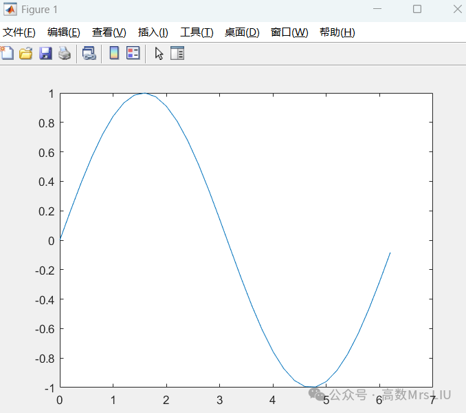
Example 1: Plotting a sine curve within [0, 2π].
x=0:0.2:2*pi; % Sampling points from 0 to 2π with a step of 0.2
y=sin(x); % Calculating the function values at the sampled points
plot(x,y) % Performing 2D plotting
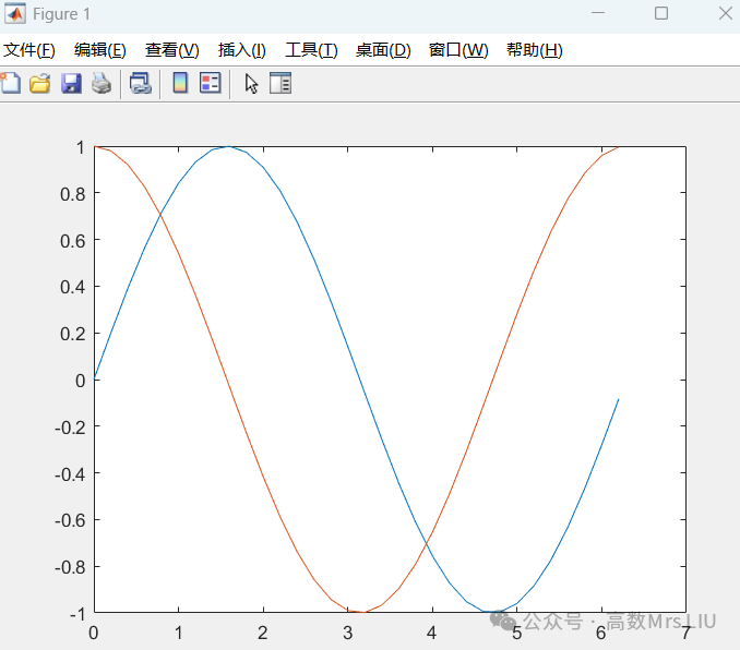
Example 2: Plotting sine and cosine curves on the same plane within [0, 2π].
x=0:0.2:2*pi; % Sampling points from 0 to 2π with a step of 0.2
plot(x,sin(x),x,cos(x)); % Performing multi-curve plotting in 2D
2. Color Marking and Control
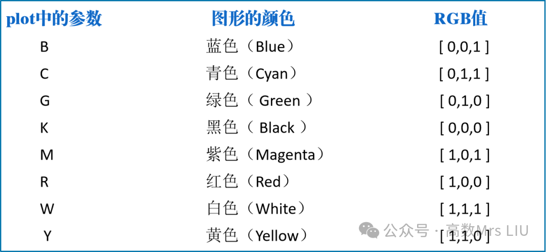
(1) Color options for the plot function
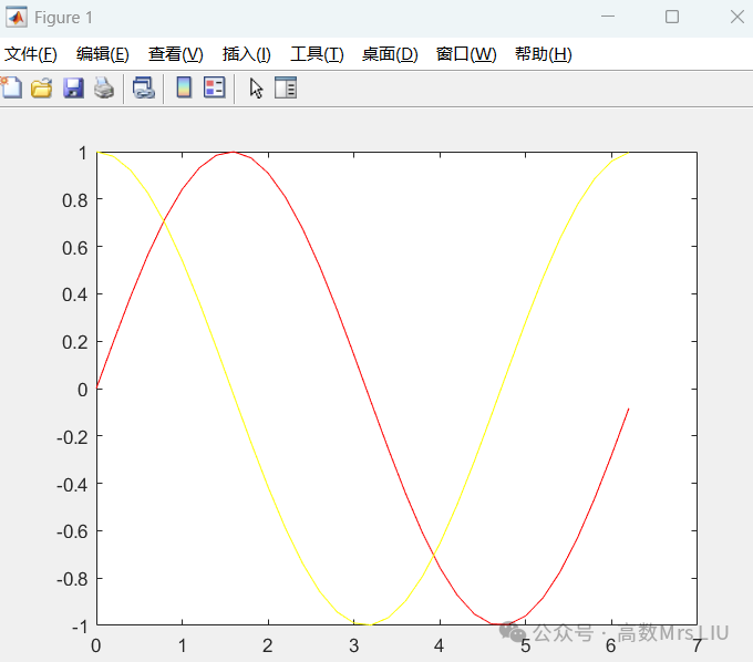
Example 1 (Color Control)
x=0:0.2:2*pi;
plot(x,sin(x), ‘r’,x,cos(x), ‘y’); % The first line is red, the second line is yellow
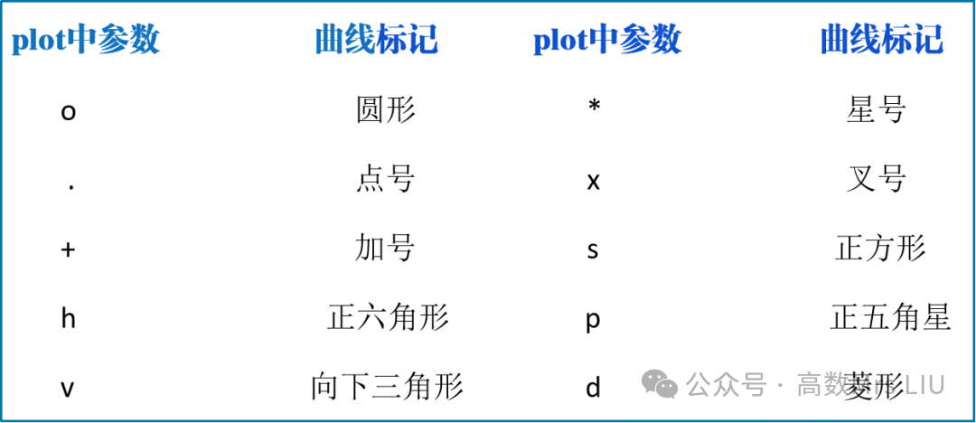
(2) Curve Marker Symbol Table
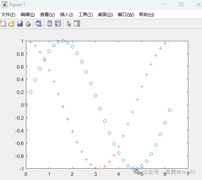
Example 2 (Marker Control)
x=0:0.2:2*pi;
plot(x,sin(x), ‘o’,x,cos(x), ‘+’); % The first line is marked with ‘o’, the second line is marked with ‘+’.
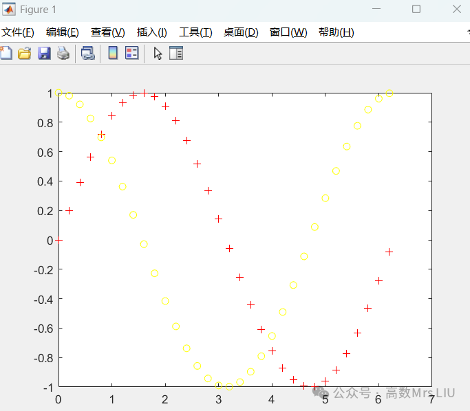
Example 3 (Simultaneous Control of Color and Markers)
x=0:0.2:2*pi;
plot(x,sin(x), ‘r+’,x,cos(x), ‘yo’); % The first line is red with ‘+’ marker,
the second line is yellow with ‘o’ marker.
(3) Curve Format Table
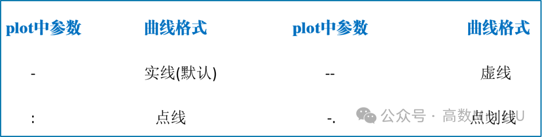
Example 4 (Control of Curve Types)
x=0:0.2:2*pi;
plot(x,sin(x), ‘r’,x,cos(x), ‘b–‘); % The first line is a solid red line, the second line is a dashed blue line.
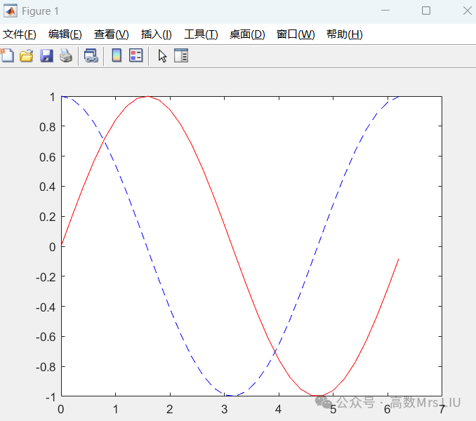
(4) Axis Control
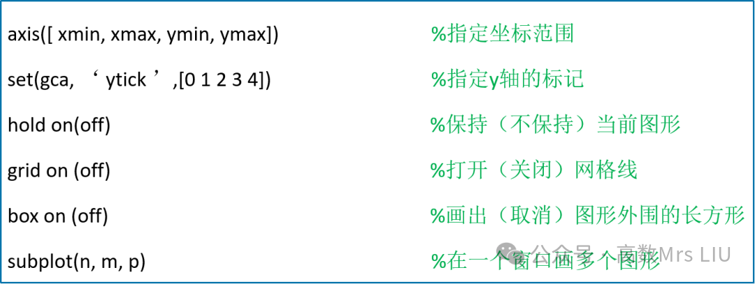
plot can automatically adjust the range and ticks of the axes based on the graph. The basic command and syntax are
 (5) Adding Text Annotations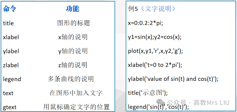
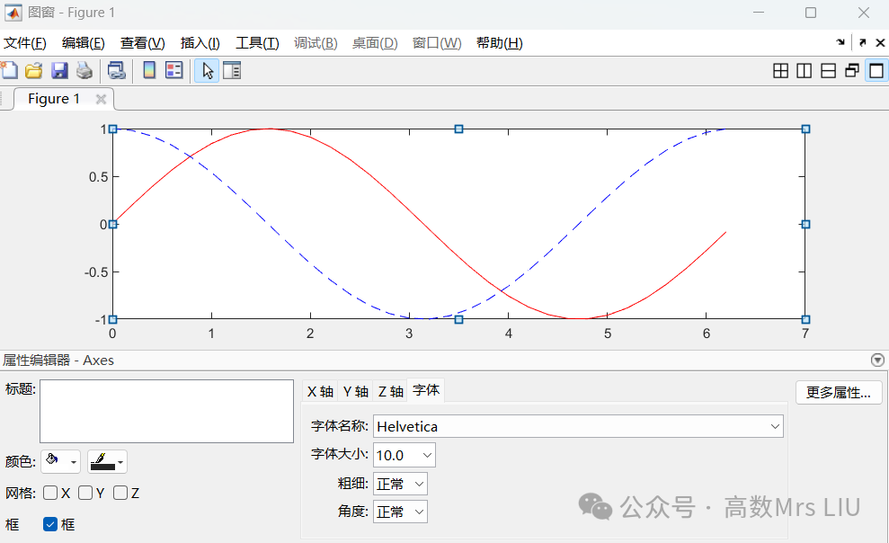
 Special Note: In addition to adding the corresponding commands during code writing to control the image, we can also directly edit in the figure window, the operation sequence is: 【View】 – 【Property Editor】.
3. Splitting the Figure Window
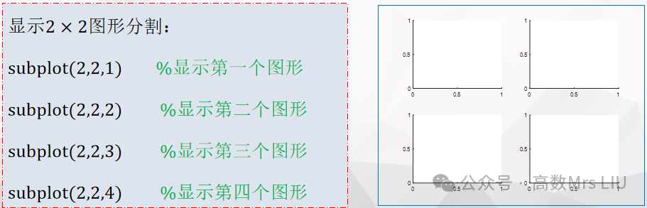
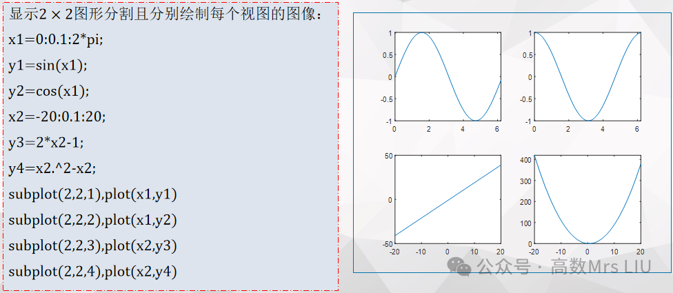
The command to split the window in Matlab is
subplot(m,n,p)
This splits the current window into m×n view areas and specifies the p-th view as the current view.
 4. Plotting in Polar Coordinates
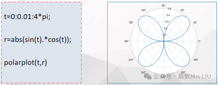
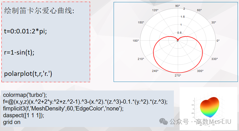
The command format to call is:
polarplot(t,r):
t represents the angle in radians, r represents the radius value for each point, and the input must be vectors of equal length or matrices of equal size.
🎀
Thank you for your attention~
I hope the above content is helpful to you!
🎀