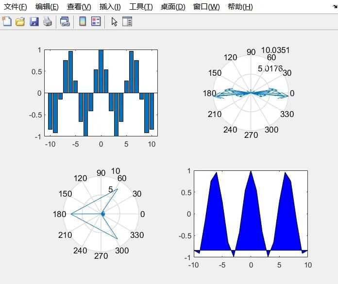
1. Bar Plot
-
t = -10:1:10;
-
subplot(2,2,1);
-
bar(t, cos(t));
Copy code
This creates a vector t containing elements from -10 to 10. In the first subplot, the bar function is used to plot the bar graph of cos(t). The first parameter of the bar function is the x-axis coordinates, and the second parameter is the height or value corresponding to each x coordinate. This subplot shows the variation of cos(t) over the given range. Compass Plot
-
subplot(2,2,2);
-
compass(t, cos(t));
Copy code
In the second subplot, the compass function is used to create a polar plot. The compass function takes t as input and cos(t) as the magnitude for the polar coordinates. This plot displays the phase and magnitude information of cos(t). Rose Plot
-
subplot(2,2,3);
-
rose(t, cos(t));
Copy code
The third subplot uses the rose function to create a rose plot. The rose function takes the angle vector t and the corresponding values cos(t), then plots the frequency corresponding to the angles on the polar axis. This figure presents the distribution of cos(t) in the form of rose petals. Filled Plot
-
subplot(2,2,4);
-
fill(t, cos(t), ‘b’);
Copy code
In the fourth subplot, the fill function is used to create a filled plot. The first parameter of the fill function is the x-axis coordinates, and the second parameter is the corresponding y values for each x coordinate. Additionally, ‘b’ indicates that blue is used for filling. This figure shows the filled effect of cos(t) over the given range. Result Screenshot Below:
-
clear
-
clc
-
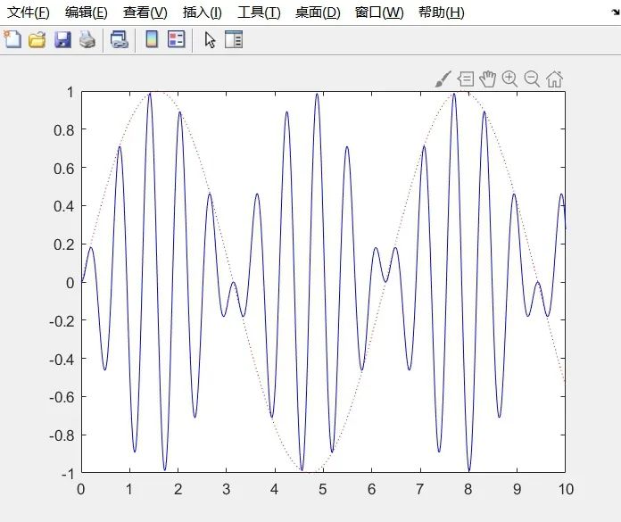
t=0:0.001:10;
-
y=sin(t);
-
% plot(t,y);
-
Y=sin(10*t);
-
c=y.*Y;
-
plot(t,y,’r:’,t,c,’b’)
Copy code
-
clear
-
clc
-
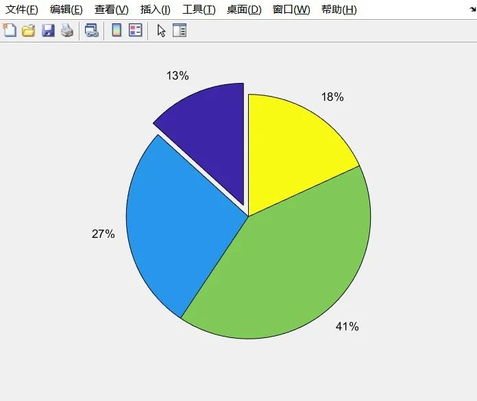
x=[11.4 23.5 35.4 15.6];
-
explode=zeros(size(x));
-
[c,offset]=min(x);
-
explode(offset)=c;
-
pie(x,explode)
Copy code
-
clear
-
clc
-
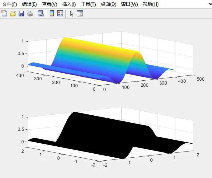
x=-2:0.01:2;
-
[x,y]=meshgrid(x,x); %x and y are both 401×401 matrices
-
r=sqrt(x.^2+x.^2)+eps;
-
z=sinc(r);
-
subplot(2,1,1);
-
mesh(z);
-
subplot(2,1,2);
-
surf(x,y,z);
Copy code
-
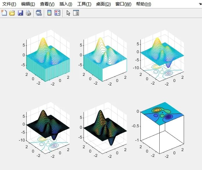
meshz function (first subplot): Plots the surface and adds a skirt, showing both the surface and the zero plane.
-
waterfall function (second subplot): Produces a water flow effect in the x direction on the surface plot.
-
meshc function (third subplot): Simultaneously draws the mesh plot and contour lines.
-
surfc function (fourth subplot): Simultaneously draws the surface plot and contour lines.
-
surfl function (fifth subplot): Provides a color surface plot with lighting effects.
-
contourf function (sixth subplot): Draws a contour filled plot, which is a contour plot with color filling.
Each subplot uses axis([-inf inf -inf inf -inf inf]) to set the display range of the axes.
-
clear
-
clc
-
[x,y,z] =peaks;
-
subplot(2,3,1);
-
meshz(x,y,z); %Surface with a skirt, showing the surface and zero plane
-
axis([-inf inf -inf inf -inf inf]);
-
subplot(2,3,2);
-
waterfall(x,y,z); %Produces a water flow effect in the x direction
-
axis([-inf inf -inf inf -inf inf]);
-
subplot(2,3,3);
-
meshc(x,y,z); %Simultaneously draws the mesh plot and contour lines
-
axis([-inf inf -inf inf -inf inf]);
-
subplot(2,3,4);
-
surfc(x,y,z); %Simultaneously draws the surface plot and contour lines
-
axis([-inf inf -inf inf -inf inf]);
-
subplot(2,3,5)
-
surfl(x,y,z); %Provides a color surface plot with lighting effects
-
axis([-inf inf -inf inf -inf inf]);
-
subplot(2,3,6)
-
contourf(x,y,z);
-
axis([-inf inf -inf inf -inf inf]);
Copy code
-
clear
-
clc
-
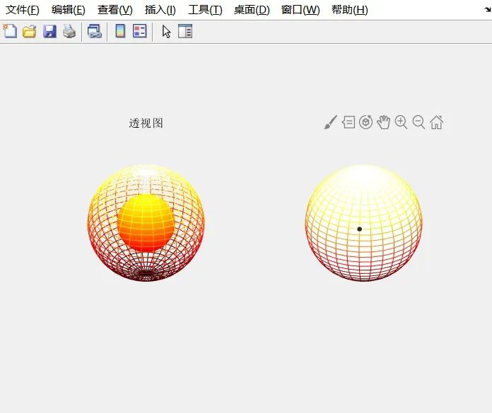
[X0,Y0,Z0]=sphere(30); %Generate three-dimensional coordinates of the unit sphere
-
X=2*X0;Y=2*Y0;Z=2*Z0; %Generate three-dimensional coordinates of the sphere with radius 2
-
clf
-
subplot(1,2,1);
-
surf(X0,Y0,Z0); %Draw the unit sphere
-
shading interp %Use interpolated shading
-
hold on,mesh(X,Y,Z),colormap(hot),hold off %Use hot colormap
-
hidden off %Generate perspective effect
-
axis equal,axis off %Do not display axes
-
title(‘Perspective View’)
-
subplot(1,2,2);
-
surf(X0,Y0,Z0); %Draw the unit sphere
-
shading interp %Use interpolated shading
-
hold on,mesh(X,Y,Z),colormap(hot),hold off %Use hot colormap
-
hidden on %Generate hidden effect
-
axis equal,axis off %Do not display axes
-
title(‘Hidden View’)
Copy code
-
clear
-
clc
-
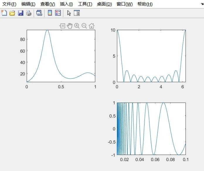
subplot(2,2,1), fplot(@humps, [0 1])
-
subplot(2,2,2), fplot(@(x) abs(exp(-1i*x*(0:9))*ones(10,1)), [0 2*pi])
-
% % Vectorize the function for subplot(2,2,3)
-
% vec_func = @(x) [tan(x),sin(x),cos(x)];
-
% x_range = linspace(2*pi*(-1), 2*pi*(1), 1000); % Adjust the number of points as needed
-
% subplot(2,2,3), fplot(vec_func, x_range)
-
subplot(2,2,4), fplot(@(x) sin(1 ./ x), [0.01 0.1], 1e-3)
Copy code
-
clear
-
clc
-
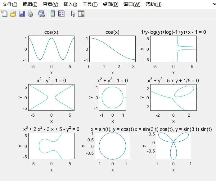
subplot(3,3,1)
-
ezplot(‘cos(x)’)
-
subplot(3,3,2)
-
ezplot(‘cos(x)’, [0, pi])
-
subplot(3,3,3)
-
ezplot(‘1/y-log(y)+log(-1+y)+x – 1’)
-
subplot(3,3,4)
-
ezplot(‘x^2 – y^2 – 1’)
-
subplot(3,3,5)
-
ezplot(‘x^2 + y^2 – 1’,[-1.25,1.25]);
-
axis equal
-
subplot(3,3,6)
-
ezplot(‘x^3 + y^3 – 5*x*y + 1/5’,[-3,3])
-
subplot(3,3,7)
-
ezplot(‘x^3 + 2*x^2 – 3*x + 5 – y^2’)
-
subplot(3,3,8)
Copy code
-
clear
-
clc
-
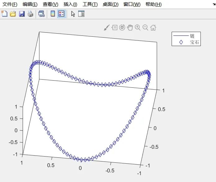
t=(0:0.02:2)*pi;
-
x=sin(t);
-
y=cos(t);
-
z=cos(2*t);
-
plot3(x,y,z,’b-‘,x,y,z,’bd’)
-
view([-82,58]);
-
box on
-
legend(‘Chain’,’Gem’);
Copy code
-
clear
-
clc
-
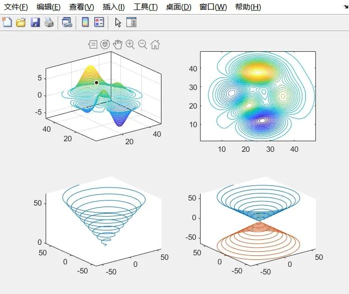
subplot(2,2,1)
-
contour3(peaks,50); %Draw contour lines of the surface in three-dimensional space
-
axis([-inf inf -inf inf -inf inf]);
-
subplot(2,2,2)
-
contour(peaks, 50); %Draw the projection of the surface contour lines on the XY plane
-
subplot(2,2,3)
-
t=linspace(0,20*pi, 501);
-
plot3(t.*sin(t), t.*cos(t), t);% Draw curve in three-dimensional space
-
subplot(2,2,4)
-
plot3(t.*sin(t), t.*cos(t), t, t.*sin(t), t.*cos(t), -t);% Simultaneously draw two curves in three-dimensional space
Copy code
-
clear
-
clc
-
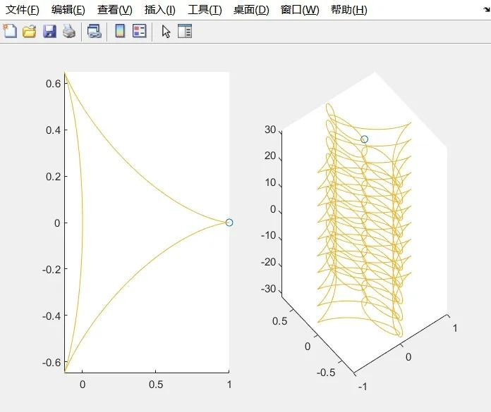
subplot(1,2,1);
-
t = 0:0.01:2*pi;
-
x = cos(2*t).*(cos(t).^2);
-
y = sin(2*t).*(sin(t).^2);
-
comet(x,y)
-
subplot(1,2,2);
-
t = -10*pi:pi/250:10*pi;
-
comet3((cos(2*t).^2).*sin(t),(sin(2*t).^2).*cos(t),t)
Copy code
Edited by / Garvey
Reviewed by / Fan RuiQiang
Checked by / Garvey
Click below
Follow us