4.5 Interpolation
Interpolation is the process of calculating estimated values between known data points. It is a practical numerical method and an important method for function approximation. Interpolation operations are widely used in signal processing and graphical analysis. MATLAB provides various interpolation functions to meet different needs.
4.5.1 One-Dimensional Data Interpolation
One-dimensional data interpolation commonly uses the function interp1, with the general syntax: yi=interp1(x,y,xi,method). Here, y is the vector of function values, x is the range of independent variable values, and the lengths of x and y must be the same; xi is the vector or array of interpolation points, and method is the option for the interpolation method. MATLAB provides the following methods for interpolation.
(1) Nearest neighbor interpolation (method=’nearest’).
(2) Linear interpolation (method=’linear’): Connects two data points with a straight line and calculates the value of the given interpolation point on the line as the interpolation result. This method is the default for the interp1 function.
(3) Cubic spline interpolation (method=’spline’): Fits a cubic spline curve through the data points and calculates the value of the given interpolation point on the curve as the interpolation result.
(4) Cubic interpolation (method=’pchip’ or ‘cubic’): Computes the interpolation result using a piecewise cubic Hermite interpolation method.
When choosing an interpolation method, factors to consider include computation time, memory usage, and the smoothness of the interpolation. Generally:
(5) The nearest neighbor interpolation method is the fastest but has the worst smoothness;
(6) The linear interpolation method uses more memory than the nearest neighbor method and has a slightly longer computation time. Unlike the nearest neighbor method, its result is continuous, but the slope at the vertices changes;
(7) The cubic spline interpolation method has the longest computation time, but its memory usage is less than that of the cubic interpolation method. Both the interpolation data and derivatives are continuous. Among these four methods, the cubic spline interpolation result has the best smoothness, but if the input data is inconsistent or the data points are too close, poor interpolation results may occur.
[Example4-39] One-dimensional interpolation function interp1 application and comparison example.
>> x=0:10;
>> y=cos(x);
>> xi=0:0.25:10;
>> strmod={‘nearest’,’linear’,’spline’,’pchip’}% Store interpolation methods in a cell array
strmod =
‘nearest’ ‘linear’ ‘spline’ ‘pchip’
>> strlb={‘(a)method=nearest’,'(b)method=linear’,…
‘(c)method=spline’,'(d)method=pchip’} % Plot labels
strlb =
Columns 1 through 2
‘(a)method=nearest’ ‘(b)method=linear’
Columns 3 through 4
‘(c)method=spline’ ‘(d)method=pchip’
>> for i=1:4
yi=interp1(x,y,xi,strmod{i}); % Interpolation
subplot(2,2,i) % Subplot
plot(x,y,’ro’,xi,yi,’b’),xlabel(strlb(i)) % Plot
end
This example creates a cell array strmod to store the 4 interpolation methods {‘nearest’,’linear’,’spline’,’pchip’}, and then uses a loop to call the interpolation function interp1. The final interpolation results are compared graphically. The comparison of one-dimensional interpolation results is shown in Figure 4-4. It can be seen that the cubic spline interpolation result has the best smoothness, while the nearest neighbor interpolation result is the worst.
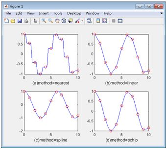
Figure 4-4 Comparison of One-Dimensional Interpolation Methods Results
4.5.2 Two-Dimensional Data Interpolation
Two-dimensional interpolation is also a commonly used interpolation operation method, mainly applied in graphical image processing and three-dimensional curve fitting. Two-dimensional interpolation is implemented by the function interp2, with the general syntax: zi=interp2(x,y,z,xi,yi,method).
Here, x and y are arrays composed of independent variables, with the same dimensions, and z is the corresponding function values; xi and yi are arrays of interpolation points, and method is the option for the interpolation method. The 4 interpolation methods in the interp1 function can also be used in the interp2 function.
[Example4-40] Two-dimensional interpolation function interp2 application and comparison example.
clear
[x,y,z]=peaks(6); % MATLAB’s built-in test function
mesh(x,y,z) % Draw original data plot
title(‘Original Data‘)
[xi,yi]=meshgrid(-3:0.2:3,-3:0.2:3); % Generate data grid for interpolation
strmod={‘nearest’,’linear’,’spline’,’cubic’}; % Store interpolation methods in a cell array
strlb={‘(a)method=nearest’,'(b)method=linear’,…
‘(c)method=spline’,'(d)method=cubic’}; % Plot labels
figure % Create new plot window
for i=1:4
zi=interp2(x,y,z,xi,yi,strmod{i}); % Interpolation
subplot(2,2,i)
mesh(xi,yi,zi); % Plot
title(strlb{i}) % Plot title
end
This example calculates interpolation using ‘nearest’, ‘linear’, ‘spline’, and ‘cubic’ methods. The original data is shown in Figure 4-5, and the results after interpolation are shown in Figure 4-6. From the result figures, it can be seen that the accuracy of various interpolation methods is different.
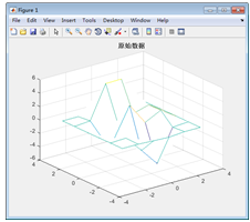
Figure 4-5 Original Data for Two-Dimensional Interpolation
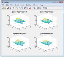
Figure 4-6 Results of Two-Dimensional Interpolation
4.5.3 Multi-Dimensional Interpolation
Multi-dimensional interpolation includes three-dimensional interpolation function interp3 and n-dimensional interpolation function interpn. The function calling methods and interpolation methods are basically the same as one-dimensional and two-dimensional interpolation. Here, taking three-dimensional as an example, its general format is:
zi=interp3(x,y,z,v,xi,yi,zi,method)
Where x, y, z are arrays composed of independent variables, with the same dimensions, and v is the corresponding function values; xi, yi, zi are arrays of interpolation points, and method is the option for the interpolation method. This is consistent with the 4 methods of one-dimensional interpolation.
[Example4-41] Three-dimensional interpolation function interp3 example.
>> [x,y,z,v]=flow(8); % flow is MATLAB’s built-in test function
>> slice(x,y,z,v,[3,5],2,[-2,3]) % Draw slice plot
>> title(‘Before Interpolation‘)
>>[xi,yi,zi]=meshgrid(0.1:0.25:10,-3:0.25:3,-3:0.25:3); % Create interpolation point data grid
>> vi=interp3(x,y,z,v,xi,yi,zi); % Interpolation
>> figure
>> slice(xi,yi,zi,vi,[3,5],2,[-2,3]) % Draw slice plot after interpolation
>> title(‘After Interpolation‘)
The flow function before interpolation is shown in Figure 4-7, and the result after three-dimensional interpolation is shown in Figure 4-8.
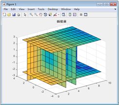
Figure 4-7 Function Plot Before Interpolation
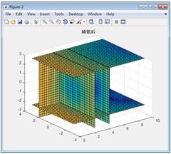
Figure 4-8 Function Plot After Interpolation
4.5.4 Spline Interpolation
The basic idea of the spline function is: given a set of known data points, the goal is to find a set of fitting polynomials. During the fitting process, for each adjacent pair of sample points (Breakpoints), a cubic polynomial is used to fit the curve between the sample points. To ensure the uniqueness of the fitting, the first and second derivatives of this cubic polynomial at the sample points are constrained. This ensures that all internal sample points have continuous first and second derivatives, except at the endpoints of the studied interval.
MATLAB provides the spline function for spline interpolation.
The calling syntax of the spline function is as follows.
(1) yy = spline(x,y,xx): Calculate the cubic spline interpolation corresponding to xx based on the sample data (x,y).
(2) pp = spline(x,y): Obtain the piecewise polynomial spline function data pp from the sample data (x,y).
[Example4-42] Spline interpolation spline function application example.
>> x = -4:4;
>> y = [0 .15 1.12 2.36 2.36 1.46 .49 .060]; % Data before interpolation
>> cs = spline(x,[0 y 0]); % Interpolation
>> xx = linspace(-4,4,101); % Create plotting independent variable array
>> plot(x,y,’o’,xx,ppval(cs,xx),’-‘); % Draw result plot
The resulting graph is shown in Figure 4-9.
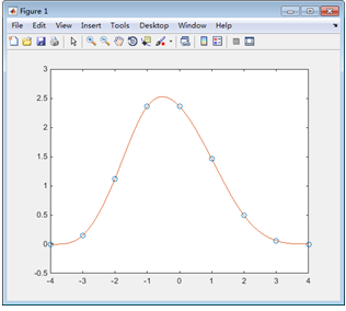
Figure 4-9 Spline Interpolation