
Source: Data STUDIO

This article is approximately 4000 words long and is recommended for a 10-minute read.

This article will systematically introduce six widely used time series smoothing techniques, analyzing them from multiple dimensions including technical principles, parameter configurations, performance characteristics, and applicable scenarios.
In time series data analysis, the issue of noise is an unavoidable challenge. Even with good signal quality, the raw data may still contain various interference factors. These noises may stem from sensor hardware defects, random errors during manual measurement, or inherent statistical fluctuations in the data itself, all of which can significantly impact the extraction of effective trend information.
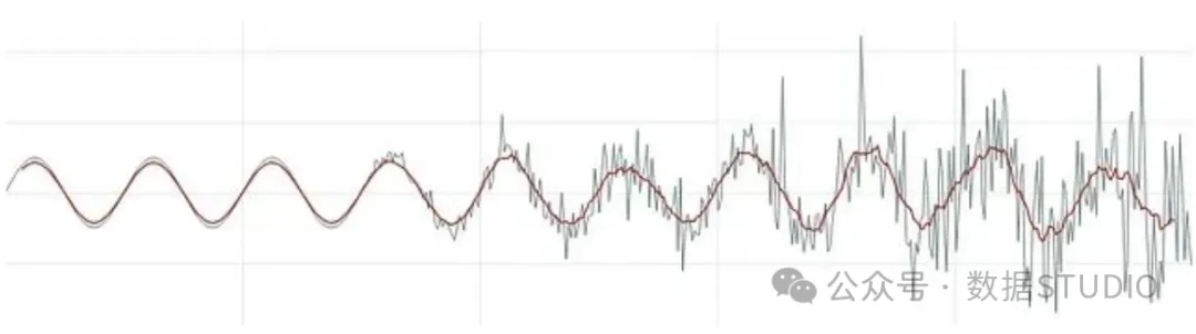
Data smoothing techniques provide an effective way to address this issue, significantly improving the interpretability and processing efficiency of the data. Choosing the appropriate smoothing method is crucial in trend identification and behavioral pattern comparative analysis, but determining the optimal method and smoothing intensity parameters often requires in-depth technical understanding.
This article will systematically introduce six widely used time series smoothing techniques, analyzing them from multiple dimensions including technical principles, parameter configurations, performance characteristics, and applicable scenarios. The article will also introduce a quantitative evaluation metric for smoothing effects and provide an interactive tool for method comparison and validation.
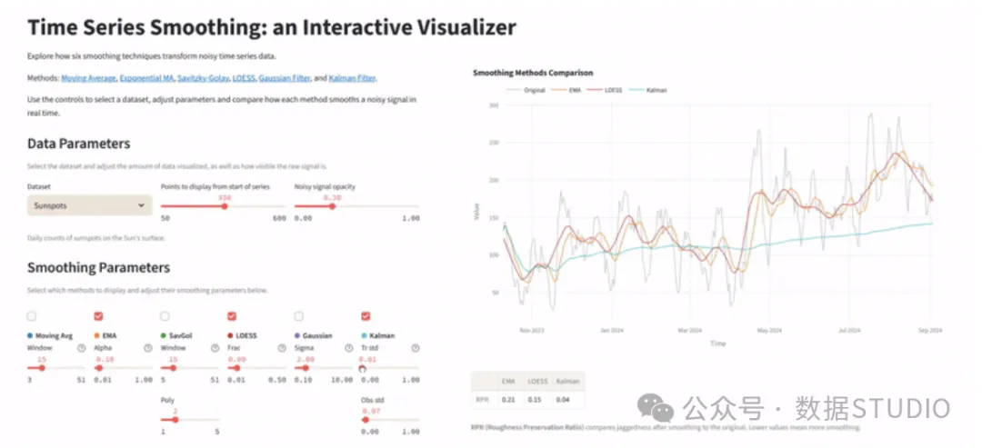
The following will detail the technical principles, core parameter configurations, and respective advantages and limitations of six mainstream smoothing methods.
Moving Average (Rolling Mean)
The moving average, also known as simple moving average, rolling window average, or sliding window average, replaces each data point in the time series with the arithmetic mean of a fixed number of neighboring data points.
The core mechanism of this method is to select a window containing surrounding data (for example, 5 data points before and after) for each target point, calculating the mean of all values within the window as the smoothed value for that point. The window size directly controls the degree of smoothing; a larger window produces a smoother curve but also increases signal delay.
The key parameter of the moving average method is the window size, which is the number of data points involved in the averaging calculation. The choice of this parameter needs to find a balance between smoothing effect and signal delay.
This method has the advantages of being simple in algorithm and high in computational efficiency, effectively eliminating short-term fluctuations and highlighting long-term trend characteristics. However, its inherent limitations include: due to the use of symmetric window calculations, it introduces a delay effect on the time axis; for sudden features such as spikes and step changes, it produces significant smoothing distortion. This method performs best when dealing with zero-mean stationary noise, that is, when data fluctuations are symmetric and statistically consistent over time.
Exponential Moving Average (EMA)
The exponential moving average employs a weighted average strategy for data smoothing, with the core feature being that more recent observations are given higher weight, allowing for a quicker response to signal changes.
The calculation process of EMA represents each new value as a weighted average of the current observation and all historical observations, with the weight coefficients decreasing exponentially. This design gives more influence to the most recent data points. EMA is a causal filter, relying only on current and historical data for calculations, making it particularly suitable for real-time data processing scenarios.
The key parameter of this method is the smoothing factor α (ranging from 0 to 1). A higher α value enhances the weight of recent observations, reducing signal delay but lowering the smoothing effect; a lower α value has the opposite effect.
Compared to the simple moving average, EMA has a faster response speed, and its causal nature ensures the feasibility of real-time processing, as it does not rely on future data for calculations. The delay introduced by EMA is relatively small compared to centered moving averages. In streaming data processing or environments with limited computational resources, EMA does not require maintaining a complete historical data window, providing significant implementation advantages. However, this method still has delay issues when processing rapidly changing signals, especially when the α parameter is small.
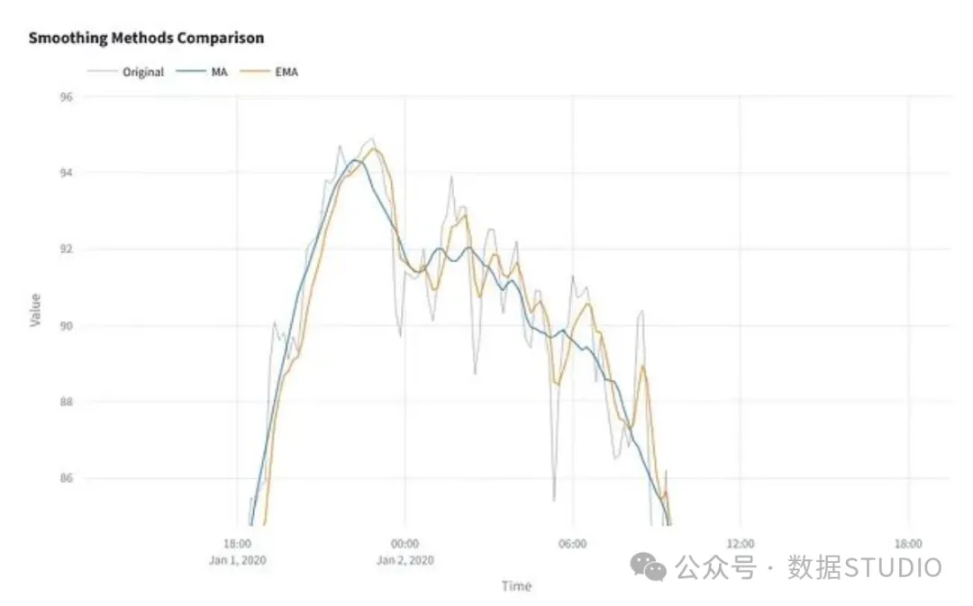
Comparison of the delay effects of moving average and exponential moving average smoothing methods.
Savitzky-Golay Filter
The Savitzky-Golay filter achieves data smoothing through local polynomial fitting. Its basic principle is to fit a low-order polynomial within a sliding data window and then replace the original data with the value of the polynomial at the center of the window. This is a local least squares regression method applied repeatedly over the time series.
The specific implementation process is: for each target point, select a symmetric data window (e.g., 11 data points), fit a polynomial of specified order (usually 2nd or 3rd) within that window, and replace the original data point with the calculated value of the fitted polynomial at the target position. This process is repeated as the window slides over the entire sequence.
This method involves two key parameters: the window size (which must be odd) determines the number of data points used for each fitting; the polynomial order controls the complexity of the local curve that the filter can represent, with higher-order polynomials able to track more complex local variation patterns.
The main advantage of the Savitzky-Golay filter is its ability to preserve high-order statistical moment features, such as slope and curvature information, making it particularly suitable for processing signals that contain structural features like peaks, valleys, or oscillations. However, when the window size is too small or the polynomial order is too high, overfitting may occur, leading to noise amplification rather than suppression.
LOESS Regression Smoothing
LOESS (Locally Estimated Scatterplot Smoothing) is a non-parametric regression method that achieves smoothing by fitting regression models to the local neighborhood of each data point. When linear fitting is used, this method is also referred to as LOWESS (Locally Weighted Scatterplot Smoothing).
The working mechanism of LOESS is: for each target point, select a certain proportion of neighboring data, assign weights based on distance, and then fit a local regression model. The smoothed value for the target point is determined by the prediction of this local model. This process is repeated across the entire time series.
The core parameter of this method is the fraction parameter (frac), which indicates the proportion of the dataset used in each local fitting. Smaller frac values make the algorithm more closely follow the local variations of the original data.
LOESS has good adaptability, capable of handling nonlinear trends and time-varying behavior patterns, maintaining good performance even when the underlying function form changes over time. Unlike the Savitzky-Golay filter, LOESS does not assume evenly spaced data or fixed structural patterns. However, this method has a higher computational complexity because it requires independent regression calculations for each data point. When the frac parameter is too small, it may lead to overfitting and noise enhancement. Additionally, due to fewer neighboring points in boundary areas, edge estimates may become unstable, and some implementations use asymmetric windows to mitigate this issue.
Gaussian Filter
The Gaussian filter achieves time series smoothing through a weighted moving average that applies Gaussian distribution weights. Unlike the simple moving average, which gives equal weight to all points within the window, the Gaussian filter assigns higher weights to data points closer to the center and lower weights to those further away, with the weight distribution following a Gaussian (normal) distribution pattern.
The implementation process of this method is: for each target point, use a symmetric Gaussian kernel function centered at that point to calculate the weighted sum of neighboring values. The shape of the kernel function is controlled by the standard deviation parameter σ, which determines the rate of weight decay but does not directly control the window size.
The key parameter of the Gaussian filter is the standard deviation σ, which controls the spread of the weight distribution. Smaller σ values maintain the responsiveness of the window, suitable for preserving signal details; larger σ values achieve broader smoothing effects.
This method can produce smooth processing results, with fewer edge effects compared to simple moving averages. When it is necessary to achieve a smoothing effect while avoiding complete flattening of the signal, the Gaussian filter is an ideal choice. This technique is widely used in image processing and signal processing fields. However, like other non-adaptive filters (moving average, EMA, Savitzky-Golay), the Gaussian filter applies a uniform smoothing strategy across the entire sequence, even in areas where the signal changes rapidly. This may lead to issues such as blurring sharp edges, flattening peaks, and delayed responses to abrupt changes.
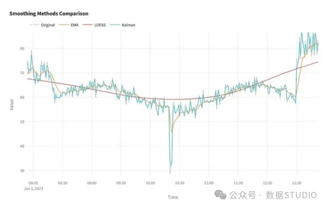
Comparison of smoothing effects of EMA, LOESS, and Kalman filter on noisy data.
Kalman Filter
The Kalman filter is a recursive estimation algorithm based on probability theory, specifically designed to estimate the underlying state of a system from noisy observation data. The algorithm predicts the state at each time step based on the process model, compares the prediction with the observation data, and then updates the state estimate to achieve an optimal balance between model prediction and actual measurement. Like EMA, the Kalman filter is also a causal smoothing method.
The Kalman filter is based on the assumption that the signal is generated by a system that follows linear dynamic laws and contains Gaussian noise. The filter simultaneously tracks two key elements: state estimate (the best estimate of the true value) and a measure of uncertainty for that estimate. When new observation data arrives, the algorithm uses a weighted average strategy to merge the predicted and observed values, with more confident estimates receiving greater weight.
This method includes two key parameters: process noise standard deviation (transition_std), which describes the noise level or unpredictability of the internal process of the system; and observation noise standard deviation (observation_std), which describes the noise level of the measurement data. These two parameters together determine the filter’s relative trust in model predictions versus new observation data.
The Kalman filter excels in handling time-varying noise and missing data, demonstrating good adaptability and smoothly tracking gradual changes. This technology is widely used in control systems, financial analysis, and sensor data fusion. However, the computational complexity of the Kalman filter is relatively high, as it requires maintaining and updating state estimates and their uncertainty information at each time step. This method requires an accurate process model, and when the actual system exhibits nonlinear, non-Gaussian, or highly irregular characteristics, the standard Kalman filter may exhibit divergence or unpredictable behavior (for nonlinear systems, variants such as the extended Kalman filter or unscented Kalman filter are needed). Additionally, the accurate tuning of noise parameters is crucial for algorithm performance; improper parameter settings may lead to over-smoothing or noise amplification issues.
Various smoothing methods have specific applicable scenarios. For applications that only require suppression of rapid fluctuations, moving averages or EMA are usually sufficient. When it is necessary to preserve signal features such as peaks and curvature, Savitzky-Golay filter or LOESS may be more suitable. The Gaussian filter is ideal for scenarios requiring smoothing effects with easy parameter tuning. Although the Kalman filter has higher complexity, it offers advantages that other methods cannot match in systems that need to adapt to dynamic changes or complex noise environments.
Technical Challenges in Practical Data Smoothing
Time series data in practical applications often exhibit complex features such as irregular sampling, missing data, and mixed rates of change. For example, IoT sensors may experience data loss or report data at uneven intervals, all of which increase the difficulty of data interpretation.
Most smoothing methods assume that data is regular and complete. When there is missing data, it may be necessary to perform interpolation or data filling beforehand, or to choose methods like the Kalman filter that can directly handle data gaps.
In streaming data or real-time processing scenarios, future data values cannot be obtained, which poses limitations for many filtering methods that rely on symmetric windows. Causal filters such as backward window moving averages, EMA, and Kalman filters are more suitable for such applications, as they only use current and historical data for state updates.
These technical challenges make parameter selection and automated result validation more difficult. Visual inspection remains the most reliable method for assessing smoothing effects. To quantitatively evaluate the degree of smoothing, we can use the following relatively simple evaluation metric:
Quantitative Analysis of Smoothing Based on RPR Metric
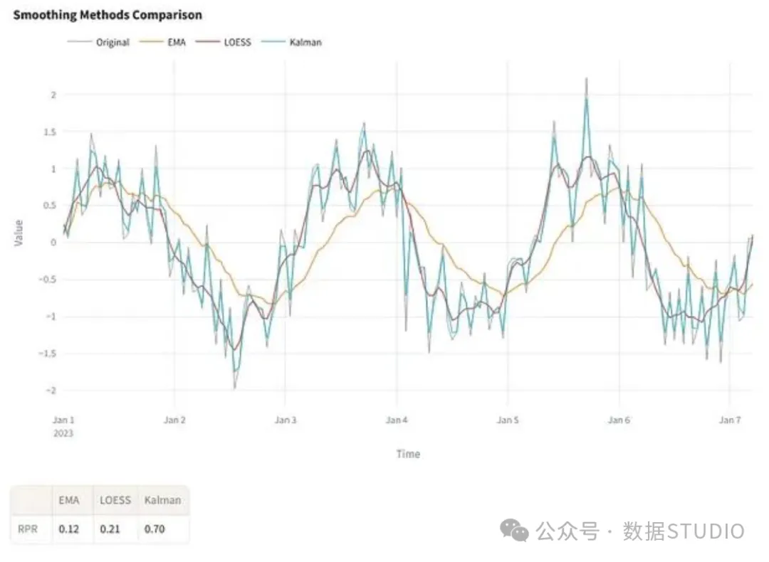
The RPR (Roughness Preservation Ratio) metric is used to quantify the degree of short-term variation retained in the signal after smoothing (i.e., “roughness”). This metric is based on total variation measurement, defined as the cumulative sum of absolute differences between consecutive data points:
RPR = ∑ |ŷᵢ₊₁ − ŷᵢ| / ∑ |yᵢ₊₁ − yᵢ|
That is:RPR = total_variation(smoothed) / total_variation(original)
The RPR value typically ranges from 0 to 1. Values close to 1 indicate lighter smoothing, while values close to 0 reflect stronger smoothing effects. When processing methods increase local variation, the RPR value may exceed 1.
It is important to note that this metric only measures the reduction of the signal’s jagged features and does not assess the preservation of the overall shape of the signal. The RPR metric is practically valuable when comparing the smoothing intensity of different methods on the same dataset.
Conclusion
Different smoothing methods exhibit significant differences in their responses to noise, trends, and structural features in time series data. No single method can achieve optimal results in all application scenarios; appropriate selection requires a comprehensive consideration of the specific requirements of data characteristics and analysis objectives.
For applications with good data quality where the main goal is to reduce minor fluctuations, simple moving averages or Savitzky-Golay filters usually provide good results. In streaming data or real-time analysis scenarios, EMA or Kalman filters may be more suitable. When signals contain nonlinear patterns or time-varying behavior features, LOESS is an excellent choice, although it has relatively high computational overhead.
The set of techniques introduced in this article has practical value but is not exhaustive. Other methods such as spline smoothing or wavelet transform-based techniques may perform better in specific applications. Result visualization is crucial for method evaluation. While metrics like RPR help compare parameter settings, graphical representation often reveals more intuitively whether methods have preserved the signal structure or caused over-smoothing.
A deeper understanding of these technical trade-offs helps avoid common pitfalls and establishes a more reliable framework for analyzing and interpreting signals.
Related code implementation can be accessed at: https://github.com/dbolotov/ts_smoothing_visualizer
Editor: Wenjing
About Us
Data Pie THU, as a data science public account, is backed by the Tsinghua University Big Data Research Center, sharing cutting-edge data science and big data technology innovation research dynamics, continuously disseminating data science knowledge, and striving to build a platform for gathering data talent, creating the strongest group in China’s big data.

Sina Weibo: @Data Pie THU
WeChat Video Account: Data Pie THU
Today’s Headlines: Data Pie THU